Pricing and hedging in the Cox-Ross-Rubinstein model

Damien LAMBERTON and Bernard LAPEYRE

July 20, 2007

Here we consider the Cox-Ross-Rubinstein model. We recall (see section

of chapter

) that

denotes the price at time

of the risky asset and for a given integer $n\geq 0$

$\begin{displaymath} S_{n+1} = S_n U_{n+1} \end{displaymath}$

where $(U_n,n\geq 1)$ is a sequence of independent random variables such that $\P(U_n=u)=p$ and $\P(U_n=d)=1-p$ where

and

are real numbers with

We denote by

the value at time

of the Cox-Ross-Rubinstein model starting from

at time

$\begin{displaymath} S^x_n = x U_1\ldots U_n. \end{displaymath}$

denote the price of the riskless asset, assumed to be given by

In computer experiments, the parameters of the model can be chosen as follows

The values of

and

will be chosen to look like a Black-Scholes model, more precisely

$\Delta t = T/N$ will be the time step for the discrete model,
$R = \exp(r* \Delta t)-1$ will be the riskless discrete interest rate on the period.

The choice of

and

are related to the discretisation of the Black-Scholes model with volatility $\sigma$ . Assuming that $\sigma=0.2$ (for a year),

and

can be chosen as (see chapter

, section

for a justification)

Describe a method to sample the vector $(S_0,\ldots,S_N)$ .
Plot typical trajectories of the Cox-Ross-Rubinstein process for different values of (from to ). Note that the price of options does not depend on the value of (see chapter ).

Scilab solution
Assuming that $d \leq R \leq u$ , show that the unique $p^\ast$ such that $\E(S_n/(1+R)^n)=1$ is given by

$\begin{displaymath} p^\ast = \frac{u-(1+R)}{u-d}. \end{displaymath}$

Why must we compute the price of an option depending on as an expectation with $p=p^\ast$ whatever the value of ?
Write an iterative algorithm allowing to compute the price of a call option with strike at time as a function
Price_at_zero(N,K,R,up,down,x).

Scilab solution

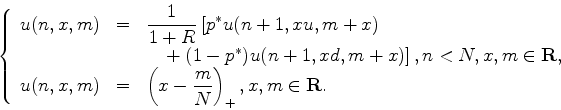
By a time shift argument write a function Price(n,N,K,R,up,down,x) which computes the price at time , when the asset value is , at this time.
Scilab solution
Compute the hedge ratio Hedge(n,N,K,R,up,down,x) at time when the asset price is using the function Price(n,N,K,R,up,down,x).
Scilab solution
Sample a trajectory $(S_n,0 \leq n \leq N)$ and check that the hedging procedure perfectly replicates the payoff whatever the value of strictly between and .
Scilab solution

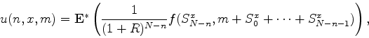
Consider an Asian call whose payoff at time is given by

$\begin{displaymath} f(S_N,S_1+\cdots+S_{N-1}) = \left(S_N - \frac{1}{N}\left(S_0+\cdots+S_{N-1}\right)\right)_+. \end{displaymath}$

Take

in numerical examples.

Using the results of chapter prove that the price at time of this option is given by

$\begin{displaymath} V_n = \frac{1}{(1+R)^{N-n}}\E^*\left(f(S_N,S_0+\cdots+S_{N-1}) \vert \F_n\right). \end{displaymath}$

Deduce from this equality that if

$\begin{displaymath} u(n,x,m) = \E^* \left(\frac{1}{(1+R)^{N-n}} f(S^x_{N-n}, m+S^x_0+\cdots+S^x_{N-n-1}) \right), \end{displaymath}$

then $V_n=u(n,S_n,S_0+S_1+\cdots+S_{n-1})$
Show that is the unique solution to

$\begin{displaymath}\left\{ \begin{array}{lcl} u(n,x,m) & = & \displaystyle \fr... ...ft(x - \frac{m}{N}\right)_+, x,m \in \R. \end{array} \right. \end{displaymath}$
Write a recursive algorithm to compute . What is the complexity of this algorithm with respect to ? Can you improve the complexity of this algorithm?
Scilab solution
Show that, between time and time , the quantity $H_{n+1}$ of risky asset in the perfect hedging portfolio is given by $H_{n+1}=h(n+1,S_n,S_0+\cdots+S_{n-1})$ where

$\begin{displaymath} h(n+1,x,m) = \frac{ u(n+1,xu,m+x) - u(n+1,xd,m+x)}{x(u-d)}. \end{displaymath}$

Scilab solution
Implement this hedging formula and check, using simulation, that it gives a perfect hedging strategy.
Scilab solution