Dam Optimal and Viable Deterministic Management

Contents

1 Problem statement and data

We consider a dam manager intenting to maximize the intertemporal payoff obtained by selling hydropower produced by water releases, when the water inflows (rain, outflows from upper dams) and the energy prices are supposed to be deterministic.

1.1 Dam dynamics

(1)

with

• time t ∈𝕋 := {t₀,…,T} is discrete (days), and t denotes the beginning of the period [t,t + 1[; we call t₀ the initial time and T the horizon;
• S(t) volume (stock) of water at the beginning of period [t,t + 1[, belonging to the discrete set , made of water volumes (h m³), where  is the maximum dam volume;
• a(t) inflow water volume (rain, etc.) during [t,t + 1[, belonging to , supposed to be deterministic, hence known in advance at initial time t₀;
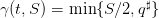
• q(t) turbined outflow volume during [t,t + 1[, decided at the beginning of period [t,t + 1[, belonging to the discrete set , where q^♯ is the maximum which can be turbined by time unit (and produce electricity), and such that

  (2)

A scenario of water inputs

(3)

is given (data of the problem), hence known in advance at initial time t₀ where the following optimization problem is posed.

1.2 Criterion: intertemporal payoff

The manager original problem is one of payoff maximization where turbining one unit of water has unitary price p(t). On the period from t₀ to T, the payoffs sum up to

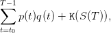(4)

where

• a scenario of prices

  (5)

  is given (data of the problem) and supposed to be known in advance at initial time t₀ where the optimization problem is posed (deterministic setting);

• the final term KS(T) is called the final value of water, since it values the water volume S(T) in the dam at the horizon T.

1.3 Numerical data

Time. We consider a daily management (the interval [t,t + 1[ represents one day) over one year

(6)

Bounds. Concerning the dam and water inflows, we consider the following bounds:

(7)

These figures reflect the assumptions that, during one week, one can release at maximum 40% of the dam volume, and that during one week of full water inflows, an empty dam can be half-filled.

Prices scenario. The scenario of prices is known in advance. We produce it by one sample from the expression

(8)

where is drawn from a sequence of i.i.d. uniform random variables in . The above expression reflects the assumption that prices are seasonal (high in winter for house heating, and low in summer).

Water inflows scenario. The scenario of water inflows is known in advance. We produce it by one sample from the expression

(9)

where is drawn from a sequence of i.i.d. uniform random variables in . The above expression reflects the assumption that water inflows are seasonal (high in winter and low in summer).

Copy the following Scicoslab code into a file DamData.sce. Check that it indeed corresponds to the data above.

2 Simulation and evaluation of given policies

First, we detail how a water turbined policy yields state (stock volume) and control (turbined) trajectories by the dynamics (1), that are then evaluated with the criterion (4). Second, you will propose different policies and you will compute their payoff.

2.1 Evaluation of a water turbined policy

An admissible policy γ : 𝕋 × 𝕏 → 𝕌 assigns a water turbined to any state S of dam stock volume and to any decision period t ∈ 𝕋, while respecting the constraints

(10)

that is,

(11)

Once given, we obtain a volume trajectory and a turbined trajectory produced by the “closed-loop” dynamics

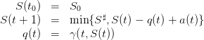(12)

and function of the scenario a(⋅) of water inputs in (3). Thus, in the end, we obtain the payoff

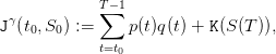(13)

as a function of the policy γ, where the trajectories  and are given by (12).

Copy the following Scicoslab code into the file DamData.sce. Check that it indeed corresponds to the expressions (12) and (13) in the special case where the final gain .

2.2 Numerical evaluation of the payoff of different policies

Load the file DamData.sce by the instruction

Copy the following Scicoslab code into a new file DamOptimality.sce. The code allows you to answer to Question 1.

Now, you will design new policies, writing code as below, following the example of the half_policy policy.

3 Dynamic programming equation

As a step towards computing an optimal water turbined policy, we provide the dynamic programming (or Bellman) equation associated with the problem of maximizing the payoff (13), as well as the corresponding Scicoslab code.

3.1 Additive dynamic programming equation

The dynamic programming equation associated with the problem of maximizing the payoff (13) is

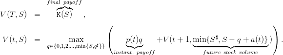(14)

Recall the definition of the characteristic function χ_A of a set A: χ_A(q) = 0 if q ∈ A, χ_A(q) = +∞ if q ⁄∈ A. Getting rid of the constraint by incorporating it in the corresponding characteristic function, the dynamic programming equation above can be written under the equivalent form

(15)

This trick will be used in the Scicoslab code. We will replace the characteristic function χ_A by a penalization: χ_A(q) = 0 if q ∈ A, χ_A(q) = 1∕𝜖 if q ⁄∈ A, where 𝜖 is a very small positive number.

3.2 Scicoslab code for the additive dynamic programming equation

Copy the following Scicoslab code into the file DamOptimality.sce. Check that it indeed corresponds to the Bellman equation (15).

4 Optimal policies

First, we will go on using a zero final value of water, meaning that leaving a stock in the dam at the end of the year is not valued. Thanks to the Scicoslab code for the Bellman equation (15), you will compute the optimal payoff and compare it with the payoffs obtained in the previous questions. Second, we will display a procedure to give proper value to a final stock. You will then compute the optimal policy and study it. At last, you will examine if this policy, designed for a single specific water inflows scenario, is sensitive to a change of scenario (robustness).

4.1 Optimal policy with a zero final value of water

We first consider that the final “value of water” is zero:

(16)

Copy the following Scicoslab code into the file DamOptimality.sce.

4.2 Computation of the final value of water

Till now, there was no gain in leaving water in the dam at the ultimate decision period as reflected in (16). Now, we consider that the final gain  is non zero, and we provide a procedure to estimate a “final value of water”, that is, a function SK(S) as in (4).

The intuition behind the procedure is that the final value of water is the value that a manager would put on the dam, were he to run it from the date T + 1 to infinity. The final value of water is the solution of an infinite horizon maximization problem. The procedure below mimicks an algorithm to find a fixed point by iterations.

First, we start with a zero final value of water and obtain, by backward induction, the Bellman function at initial time. Up to a translation — to account for the fact that an empty dam has zero final value of water — we identify with the new final value of water . Proceeding along, we expect that this loop converges towards a function SK^(∞)(S) which is a good candidate for the final value of water.

We design a loop for k = 1,…,K, starting with a zero final value of water

(17)

then solving the backward Bellman equation

(18)

then closing the loop by choosing the new final value of water

(19)

as the Bellman function at the initial time t₀ after translation, so that .

Copy the following Scicoslab code into the file DamOptimality.sce.

4.3 Optimal policy with a non zero final value of water

Copy the following Scicoslab code into the file DamOptimality.sce.

4.4 Robustness with respect to water inflows scenarios

The optimal policy discussed in Question 5 is taylored for one single inflows scenario. We now want to figure out how it responds to other inflows scenarios.

5 Optimal and viable management with guaranteed minimal volume during Summer months

For “tourism” reasons, the following viability constraint is imposed on the stock volume during some Summer months:

(20)

Such a state constraint can be treated by dynamic programming by incorporating it in the corresponding characteristic function.

The viability constraint (20) is an additional constraint, hence reduces the domain of optimization. Therefore, the payoff is lower.

References