Abstract
In this practical work, you will solve a toy stochastic control problem using the dynamic programming algorithm.
We consider a control system given by the dynamics
|
| (1) |
where
 , where
 | (2) |
where we call ti the initial time and tf the horizon;
 | (3) |
where x♯ ≥ 5 is an integer;
 | (4) |
 | (5) |
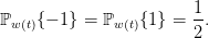
and we assume that
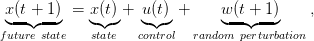
The manager is supposed to make a decision u(t) at each t ∈ 𝕋, at the beginning of the period [t,t + 1[, before knowing the random perturbation w(t + 1): such a setup is called decision-hazard setting. As the random perturbation w(t + 1) comes after the decision u(t), it might be that the future state x(t + 1) in (1) goes outside the state set 𝕏. Therefore, at the boundaries 1 and x♯ ≥ 5 of the state set 𝕏, we have to limit the set of possible controls to ensure that the future state will remain in the prescribed bounds.
Question 1
Let xref ∈ 𝕏 be a given reference state to be achieved at horizon time tf. The aim of the manager is to minimize the final cost
 | (7) |
For this purpose, the manager can select among admissible (state) policies. An admissible policy is a mapping γ : 𝕋 × 𝕏 → 𝕌 that assigns an admissible control to any time and state, that is, γ(t,x) ∈ 𝔹(x), for all (t,x) ∈ 𝕋 × 𝕏.
Let xi ∈ 𝕏 be a given initial state. The stochastic control problem to solve is now
 | (8) |
subject to the dynamics (1) and constraints that
 | (9) |
We take
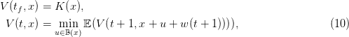
Since the perturbations w(ti + 1),…,w(tf) are supposed to be independent random variables, Dynamic Programming applies and the equation associated with the problem of minimizing the expected cost (14) writes
for time t varying from tf − 1 to ti. The expectation 𝔼 is taken with respect to the marginal probability distribution ℙw(t+1) given by (6).
vu = 0
;
for
w ∈ 𝕎 do
vu = vu + 
 V (t + 1,x + u + w)
 ;
;
if vu < V (t,x) then
Algorithm 1: Dynamic programming algorithm corresponding to (10)
Writing the code to compute the Bellman function V in (10) (and the optimal control) follows a standard scheme, sketched in Algorithm 1. In the simple example of §1.1, we directly store the Bellman values in a 2-indices matrix V = (V (t,x))t∈[ti,tf],x∈𝕏.
Question 2
Question 3 [3] Modify the previous code in order to also keep track of the optimal control function. As for the Bellman value function, you will use a 2-indices matrix U = (U(t,x))t∈[ti,tf−1],x∈𝕏 to store the optimal control at time t when the current state is x. Display the matrix U. Do you find the optimal policy intuitive?
Note that, if we know the Bellman function V , we can use Equation (10) to compute the optimal
control  to be used for a given state x at time t by
 | (11) |
This way of doing is used when Bellman functions are computed on grids, but that the system dynamics produce states outside the grid. In that case, we use interpolation to compute Bellman values and we obtain better controls by recomputing them from Equation (10), than by using stored controls associated with states limited to the grid.
As defined in §1.1, an admissible policy γ : 𝕋 × 𝕏 → 𝕌 is such that γ(t,x) ∈ 𝔹(x). The optimal control obtained by dynamic programming is an admissible policy.
Given an admissible policy γ and a (perturbation) scenario w(⋅) =  w(ti + 1),…,w(tf)
 , we are
able to build a state trajectory x(⋅) =
, we are
able to build a state trajectory x(⋅) =  x(ti),…,x(tf − 1),x(tf)
 and a control trajectory
u(⋅) =
and a control trajectory
u(⋅) =  u(ti),…,u(tf − 1)
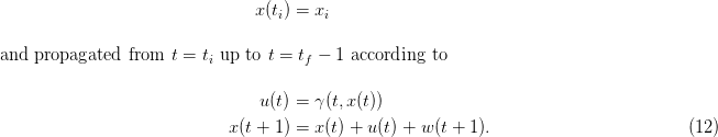
 produced by the “closed-loop” dynamics initialized at the initial time ti
by
produced by the “closed-loop” dynamics initialized at the initial time ti
by
We also obtain the payoff associated with the scenario w(⋅)
 | (13) |
where x(⋅) and u(⋅) are given by (12). The expected payoff associated with the policy γ is
 | (14) |
where the expectation 𝔼 is taken with respect to the product probability ℙ,
whose marginals are given by (6). The true expected value (14) is difficult to
compute,1
and we evaluate it by the Monte Carlo method using Ns scenarios  w1(⋅),…,wNs(⋅)
 :
:
 | (15) |
By the law of large numbers, the mean payoff (15) is a “good” approximation of the expected payoff(14) if the number of scenarios is “large enough”.
We propose three different functions in order to evaluate the mean payoff associated with a policy given by a macro named policy.
The first version uses a Monte Carlo approach. The third argument of the function N is the number of requested simulation for Monte Carlo.
The second version uses the law of the random perturbations to compute the expectation.
The third version uses dynamic programming.
Question 5 [4] Use the proposed simulation macros to evaluate the mean payoff associated with the optimal policy in (11). Compare the different proposed solutions.