Contents
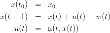
Let time t be measured in discrete units (such as days, weeks or months). Consider the
inventory problem
 | (1) |
where
- time t ∈{t0,…,T} is discrete,
- x(t) is the stock at the beginning of period t, belonging to
 ,
,
- u(t) is the stock ordered at the beginning of period t, belonging to
 ,
,
- w(t) is the uncertain demand during the period t, belonging to
 .
.
When x(t) < 0, this corresponds to a backlogged demand, supposed to be filled immediately once
inventory is again available.
1 Expected costs minimization
(Bertsekas, 2000)
The manager problem is one of cost minimization where
- ordering stock has unitary purchasing cost c,
- unitary shortage cost for unfilled demand is b,
- unitary holding cost for excess inventory is h.
The costs incurred in period t are
 | (2) |
For simplicity, we shall denote
 | (3) |
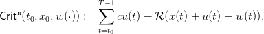
On the period from t0 to T, the costs sum up to
![T∑−1
[cu(t) + ℛ (x(t) + u(t) − w (t))].
t=t
0](inventory_control6x.png) | (4) |
We shall suppose that unitary costs are ranked as follows:

We suppose that w(t), the uncertain demand, is a random variable with distribution
 on the set
  :
:
 | (5) |
We also suppose that the random variables
 | (6) |
are independent.
A decision rule 𝔲 : ℕ × 𝕏 → 𝕌 assigns a (stock) order  to any state
x of inventory stock and to any period t. Once given, we obtain random trajectories
to any state
x of inventory stock and to any period t. Once given, we obtain random trajectories
and thus random costs
 | (7) |
The expected costs are
![T∑−1
𝔼[Crit𝔲(t0,x0,w (⋅))] = 𝔼[ cu(t) + ℛ (x(t) + u(t) − w (t))].
t=t0](inventory_control15x.png) | (8) |
The dynamic programming equation associated to the problem of minimizing the expected costs
is
![(
|| V (T,x ) = 0 ,
{ fi◟n◝al◜◞cost
V (t,x ) = inf 𝔼[(cu + ℛ (x + u − w) +V (t + 1,x + u − w ))],
||( u≥0 ◟-------◝◜-------◞ ◟---◝◜---◞
instantaneous cost future stock](inventory_control16x.png) | (9) |
where w is a random variable with the distribution  on the set
  .
.
We have that
![∑N
V (T − 1,x) = iun≥f0𝔼 [cu + ℛ (x + u − w )] = inuf≥0[cu + piℛ (x + u − i)].
i=0](inventory_control19x.png) | (10) |
Question 1 Recalling that  , show that
 ![g(z) = 𝔼[cz + ℛ (z − w )]](inventory_control21x.png) is a convex
function with a minimum achieved at some ST−1 ∈{0,…,N}. You can draw a graph of the
above function for N = 1 and p0 = 1∕2.
is a convex
function with a minimum achieved at some ST−1 ∈{0,…,N}. You can draw a graph of the
above function for N = 1 and p0 = 1∕2.
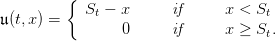
Observe that ![𝔼[cu + ℛ (x + u − w)] = − cx + g(x + u)](inventory_control22x.png) , and deduce that the optimal rule
is
, and deduce that the optimal rule
is
 | (11) |
Interpret this rule, sometimes called base-stock policy.
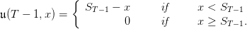
Question 2 Show by induction that there exist thresholds  in {0,…,N} such that
the optimal rule at period t is
in {0,…,N} such that
the optimal rule at period t is
 | (12) |
We know will make numerical simulations, and try different rules.
Question 3 Sample one random sequence of T − t0 demands with the macro grand.
Picture the trajectories of the stocks corresponding to the constant decision rule  .
Evaluate the costs as in (4).
.
Evaluate the costs as in (4).
purchasing=100;
shortage=150; holding=20; function c=SHcosts(zz)
c=shortage*maxi(-zz,0)+holding*maxi(zz,0); endfunction
function c=instant_costs(xx,uu,ww) c=purchasing*uu+SHcosts(xx+uu-ww); endfunction
function u=constant_rule(t,x) u=2; endfunction
function [XX,UU,CC]=trajectories(simulations,rule) XX=[]; UU=[]; CC=[];
WW=grand(horizon,'markov',transition,ones(1,simulations)); for s=1:simulations do xx=0;
uu=[]; cc=0; ww=WW(s,:); for t=0:(horizon-1) do uu=[uu,rule(t,xx($))];
xx=[xx,xx($)+uu($)-ww(t+1)]; cc=cc+instant_costs(xx($),uu($),ww(t+1));
end XX=[XX;xx]; UU=[UU;uu]; CC=[CC;cc];
end disp('expected costs are '+string(mean(CC))); endfunction horizon=12;
proba=0.01*[40,20,30,10];
transition=ones(proba')*proba; simulations=1;
simulations=100; simulations=10;
xset("window",21);xbasc(); [XX,UU,CC]=trajectories(simulations,constant_rule);
plot2d(0:horizon,XX') constant_rule_costs=mean(CC)
Question 4 Draw 100 random sequences of T −t0 demands. Picture the trajectories of the
stocks corresponding to the constant decision rules  , for k = 0, 1, 2, 3. What do
you observe? Evaluate the expected costs by Monte Carlo. What is the optimal rule among
the constant decision rules?
, for k = 0, 1, 2, 3. What do
you observe? Evaluate the expected costs by Monte Carlo. What is the optimal rule among
the constant decision rules?
simulations=1; simulations=100;
[XX,UU,CC]=trajectories(simulations,constant_rule); plot2d(0:horizon,XX')
constant_rule_costs=mean(CC)
Question 5 Picture the trajectories of the stocks corresponding to the following optimal
decision rule. Compare these trajectories with those obtained with the constant decision rules
above. What do you observe? Evaluate the expected costs by Monte Carlo. Compare with the
expected costs given by the best constant decision rule.
function [FEEDBACK,state_min]=SDP() states=[(mini(controls)-maxi(demands))*(horizon): ...
(maxi(controls)-mini(demands))*(horizon)];
cardinal_states=prod(size(states)); cardinal_controls=prod(size(controls));
cardinal_demands=prod(size(demands)); state_min=mini(states);
state_max=maxi(states); function i=index(x) i=x-state_min+1; endfunction
function xdot=dynamics(x,u,w) xdot=maxi(state_min,mini(state_max,x+u-w));
endfunction VALUE=zeros([0:horizon]'*states); FEEDBACK=zeros([0:horizon]'*states);
VALUE(horizon+1,:)=zeros(states); shift=1+[(horizon-1):(-1):1];
for tt=shift do loc=zeros(cardinal_controls,cardinal_states);
for jj=1:cardinal_controls do uu=controls(jj); loc(jj,:)=0;
for dd=1:cardinal_demands do
ww=demands(dd); loc(jj,:)=loc(jj,:)+ ...
proba(dd)* ... (instant_costs(states,uu,ww)+ ...
VALUE(tt+1,index(dynamics(states,uu,ww)))); end; end
[mmn,jjn]=mini(loc,'r'); [mmx,jjx]=maxi(loc,'r');
VALUE(tt,:)=mmn;
FEEDBACK(tt,:)=controls(jjn); end endfunction horizon=12;
proba=0.01*[40,20,30,10]; transition=ones(proba')*proba; demands=[0:(prod(size(proba))-1)];
controls=[0:2*(prod(size(proba)))]; [FEEDBACK,state_min]=SDP();
function u=optimal_rule(t,x) tt=t+1; u=FEEDBACK(tt,x-state_min+1); endfunction
xset("window",22);xbasc();
[XX,UU,CC]=trajectories(simulations,optimal_rule); plot2d([0:horizon],XX')
xtitle("Stock trajectories (minimal cost)"); optimal_costs=mean(CC)
Question 6 Increase the unitary holding cost h and decrease the unitary shortage cost b.
What do you observe?
Question 7 Decrease the horizon T to T = 4 and the maximal demand to 2. Examine the
matrix FEEDBACK. Show that the optimal rule is the form (12). What are the values of the
thresholds  ?
?
horizon=4; proba=0.01*[40,20,40]; demands=[0:(prod(size(proba))-1)];
controls=[0:10]; [FEEDBACK,state_min]=SDP();
Question 8 Suppose now that there is a fixed cost K > 0 for ordering stock. Simulate
optimal trajectories of the stocks and of the controls. What do you observe for the controls
trajectories?
K=30; function c=instant_costs(xx,uu,ww)
c=K*sign(uu)+purchasing*uu+SHcosts(xx+uu-ww); endfunction
2 Stochastic viability
(De Lara and Doyen, 2008)
Now, the manager aims at maximizing the probability
 | (13) |
that stocks are above a critical level  (to limit unsatisfied clients) and that purchasing and
holding costs are bounded above by C♯.
(to limit unsatisfied clients) and that purchasing and
holding costs are bounded above by C♯.
The dynamic programming equation associated is
![(
{ V (T,x) = 1
( V(t,x) = sup 𝔼[1{x≥x♭}1 {cu+h max{0,x+u−w}≤C ♯} × V (t + 1,x + u − w)],
u≥0](inventory_control32x.png) | (14) |
where w is a random variable with the distribution  on the set
  .
.
function [FEEDBACK,state_min]=SVSDP() states=[(mini(controls)-maxi(demands))*(horizon): ...
(maxi(controls)-mini(demands))*(horizon)]; cardinal_states=prod(size(states));
cardinal_controls=prod(size(controls)); cardinal_demands=prod(size(demands));
state_min=mini(states); state_max=maxi(states); function i=index(x) i=x-state_min+1;
endfunction function xdot=dynamics(x,u,w) xdot=maxi(state_min,mini(state_max,x+u-w));
endfunction VALUE=zeros([0:horizon]'*states); FEEDBACK=zeros([0:horizon]'*states);
VALUE(horizon+1,:)=ones(states); shift=1+[(horizon-1):(-1):1];
for tt=shift do loc=zeros(cardinal_controls,cardinal_states);
for jj=1:cardinal_controls do uu=controls(jj); loc(jj,:)=0;
for dd=1:cardinal_demands do
ww=demands(dd); loc(jj,:)=loc(jj,:)+ ...
proba(dd)* ... (bool2s(states >= stockflat) .* ...
bool2s((purchasing*uu+holding*maxi(states+uu-ww,0)) <= costsharp) .* ...
VALUE(tt+1,index(dynamics(states,uu,ww)))); end; end
[mmn,jjn]=mini(loc,'r'); [mmx,jjx]=maxi(loc,'r');
VALUE(tt,:)=mmx;
FEEDBACK(tt,:)=controls(jjx); end
endfunction horizon=12; proba=0.01*[40,20,30,10]; transition=ones(proba')*proba;
demands=[0:(prod(size(proba))-1)]; controls=[0:2*(prod(size(proba)))];
stockflat=-2; costsharp=1000; [FEEDBACK,state_min]=SVSDP();
function u=optimal_viable_rule(t,x) tt=t+1; u=FEEDBACK(tt,x-state_min+1);
endfunction
xset("window",23);xbasc(); [XX,UU,CC]=trajectories(simulations,optimal_viable_rule);
plot2d([0:horizon],XX') xtitle("Stock trajectories (maximal viability probability)");
References
D. P. Bertsekas. Dynamic Programming and Optimal Control. Athena Scientific,
Belmont, Massachusets, second edition, 2000. Volumes 1 and 2.
M. De Lara and L. Doyen. Sustainable Management of Natural Resources. Mathematical
Models and Methods. Springer-Verlag, Berlin, 2008.