Ut − D
tUt +W
t+1Et s E
t+1l
Ut − D
tUt +W
t+1Et s E
t+1l
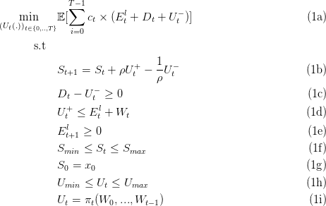
Figure 1: Electrical problem representation
Power Line Icon made by Freepik from www.flaticon.com is licensed by Creative Commons BY 3.0
Abstract
In this practical work, you will have to manage a battery in order to recover subways braking electrical energy and to supply it to a subway station. Your goal is to minimize the cost of energy consumed on the national grid by exploiting optimally this regenerative braking energy. First you will compute the gains realized when the battery is controlled according to an intuitive strategy. Then you will compare two methods, Stochastic Dynamic Programming and Model Predictive Control. Both methods provide a control for the battey at each time step these methods don’t use the same amount of information about the past randomness realization. And they don’t use their information the same way. You will compare throughout this work different ways to use past information to compute controls aware of the future uncertainties.
Subway stations represent one third of the Paris subway system energy consumption. There are unexploited energy ressources in subway stations that could be harvested to lower this energy consumption. We could for example recover braking energy from the trains. Currently trains can dissipate their kinetic energy by braking mechanically or convert this energy into electricity. However supply/demand equilibrium have to be ensured on the subway line. Hence a train can brake electrically only if there is a train accelerating/consuming energy nearby. There is therefore a significant amount of potential energy that is currently wasted. We could overcome this problem with an electrical storage.
We consider a subway station equiped with a battery that can charge braking energy and national grid energy on one side (subway line side) and discharge energy to power the subway station which is also powered by the national grid (subway station side). A battery manager has to control this battery in real time. The station demand and the cost of electricity are assumed deterministic. Braking energy available at each time step is uncertain.
Ut − D
tUt +W
t+1Et s E
t+1l
We present hereby the stochastic optimization problem we want to solve:
We detail all notations and equations in the following.
The battery can store power coming from the trains or the national grid and supply power to the subway station. It cannot do both things at the same time. We control its state of charge (soc). We model the dynamics of the battery at each time step t by a function ft we call the dynamic at time t giving equation (1b) :

where
The initial state of charge of the battery is called x0 and appears in the equality constraint (1g)
We define hereby the remaining variables of the problem presented in figure1
We observe that charge/discharge decision Ut is taken at the beginning of [t,t + 1[, before knowing the available braking energy Wt. We are in a decision-hazard setting.
We have to ensure the supply/demand equilibrium at each node and each time step on the subway station node which leads to equation:
 | (2) |
On the subway line node we have to ensure supply/demand balance however we are not forced to recover all the regenerative braking energy Wt. We have then an inequality constraint (1d):
 |
We prevent the battery manager to sell power to the grid then we have to ensure:
At each time t we pay to the national grid operator the quantity Etl + E ts of energy. We assume that the price of electricity ct per kWh is known in advance as it is negociated and constant during [t,t + 1[.
At each time t we pay the instantaneous cost:
 |
Using equation (2) we can eliminate the variable Ets leading to the instantaneous cost:
 |
At the end of the horizon we have no preference concerning the final state of charge of the battery. We introduce then a final cost function K : 𝕏 → ℝ such as:
 |
From 0 to T the payoffs sum up to:
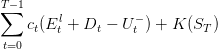 | (3) |
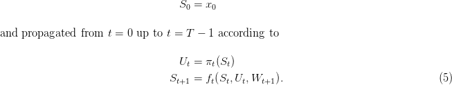
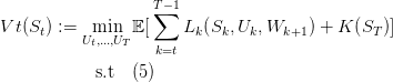
The manager wants to minize these payoffs every day without knowing the future availability of braking energy. He will therefore minimize them on average, hopefully obtaining the best mean payoff he can obtain after several days. The manager wants to minimize the expected payoff:
![T∑−1
𝔼 [ c (El + D − U −) + K (S )]
t t t t T
t=0](subway_stations_energy_management13x.png) | (4) |
The manager wants to solve problem (1). We detail the last constraint (1i) in the following.
We define, in file constants.jl, some numerical data required to model the problem.
Question 1 Comment each line by defining the constant after the #. What is the number of time steps of the problem? The number of time steps in one hour? Include the file constants.jl in your script or notebook. Plot the cost of electricity as well as the consumption of the station during the day. Compute the cost of the station’s energy consumption over the whole time horizon when it consumes exclusively on the national grid.
We provide a code function, defined in scenarios_generation.jl , that allows to compute a given number of braking energy scenarios over the time horizon.
Question 2 Include scenarios_generation.jl in your script or notebook. Use this function to generate 50 regenerative braking scenarios and save the 2 outputs. The first output contains the braking energy scenarios, we leave the second output until the end. Based on this 50 scenarios what is the average energy available over a day? We will call these 50 scenarios the assessment scenarios thoughout the work. We will refer to the second output as the ξ-assessment scenarios.
We define here 4 code functions required to model the problem.
Question 3 What is the number of state variables? What is the number of control variables? Verify that the code functions correspond the real functions of the problem.
The manager wants to be able to make a decision that takes into account the future uncertainties but that use the information about the past uncertainties realization. This is the meaning of the last constraint (1i) of problem (1) we did not yet explained.
The constraint Ut = πt(W0,...,Wt−1) states that the decision at time t, Ut, must depend only on the past uncertainties of the problem W0,...,Wt−1.
When the Wt are time independent we can restrict the search to functions of the current state of the problem. The non anticipativity constraint becomes Ut = πt(St). When the Wt are not time independent we can still restrict the search to functions of the state. The controls obtained are not guaranteed to be optimal but they may be good enough and are often easier to compute.
An admissible state feedback policy π : 𝕋 × 𝕏 → 𝕌 assigns a charge or discharge
instruction Ut = πt(St) ∈ 𝕌 to any time t ∈ 𝕋 and to any state of charge St ∈ 𝕏,
while respecting the problem constraints. Given an admissible policy π and given a
braking energy scenario W(⋅) =  W0,…,WT−1
 , we are able to build a battery state of
charge trajectory S(⋅) :=
, we are able to build a battery state of
charge trajectory S(⋅) :=  S0,…,ST−1,ST
  and a charge/discharge control trajectory
U(⋅) :=
and a charge/discharge control trajectory
U(⋅) :=  U0,…,UT−1
 produced by the “closed-loop” dynamics initialized at the initial time 0
by
produced by the “closed-loop” dynamics initialized at the initial time 0
by
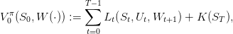
We also obtain the payoff associated to the braking energy generation scenario W1,...,WT :
 | (6) |
where S(⋅) and U(⋅) are given by (5).
The expected payoff associated with the policy π is
 | (7) |
where the expectation 𝔼 is taken with respect to the product probability ℙ. The true expected value (7) is
difficult to compute,1
and we evaluate it by the Monte Carlo method using Ns braking energy scenarios  W1(⋅),…,WNs(⋅)
 :
:
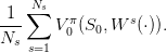 | (8) |
By the law of large numbers, the mean payoff (8) is a “good” approximation of the expected payoff(7) if the number of scenarios is “large enough”.
We propose here a code function providing a heuristic strategy base only on state and time
information. At time t this function return a control ut knowing t and xt. This code function is
then a state feedback. Its idea is to charge during peak hours and discharge during off-peak hours
while ensuring the state and control constraints.
Question 4 What are the peak and off-peak hours? What is the sign of the control returned by this heuristic according to the time at which it is computed? Explain the logic of this heuristic.
We provide a code function, in policy_assessment.jl, to assess a policy along multiple scenarios knowing the instantaneous cost, the final cost, the dynamic, the scenarios, the initial state of the system and the policy.
Question 5 Use this function with the previous heuristic on each on the assessment scenarios. What is the average cost of energy consumption on the national grid obtained? Compare with the origanl cost when there was no battery. Plot the battery state of charge for some scenarios. Does it correspond to your previous understanding of the heuristic?
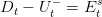
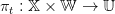
Stochastic Dynamic Programming is a method to solve Stochastic Optimal Control problems. It is based on the concept of value functions and the so called Bellman’s principle of optimality. The value function of the problem at time t is defined as:
With K the final cost of the problem which is zero in our case. The principle of optimality states that, when the problem noises are independent, we can write the following recursion between value functions:
![Vt(St ) = min 𝔼[Lt(St,Ut,Wt+1 ) + Vt+1 (ft(St,Ut,Wt+1 ))]
Ut](subway_stations_energy_management27x.png) | (9) |
In practice we use equation (9) in two phases: an offline stage where we use it to compute value functions, and an online stage where these functions are used to compute a control.
Offline phase: computation of value functions
For t from T to 0 compute
![Vt(St) = min 𝔼[Lt(St,Ut,Wt+1 ) + Vt+1 (ft(St,Ut,Wt+1 ))]
Ut∈𝕌](subway_stations_energy_management28x.png) | (10) |
Online: computation of a control
At time t, knowing the state of the system St compute Ut:
![Ut ∈ arg min 𝔼 [Lt(St,U, Wt+1 ) + Vt+1(ft(St,U, Wt+1))]
U ∈𝕌](subway_stations_energy_management29x.png) | (11) |
In practice we compute the value functions on a discretized state space 𝕏d. As it is not possible to iterate over a continuous set. Similarly we solve problems (19) and (20) by discretizing 𝕌 and testing every control in 𝕌d the discrete space obtained.
In order to compute the expectation in problems (19) and (20) we assume that the noises are time independent and use 1000 braking energy scenarios to compute the marginal laws of the noises at each time step. We do not use the assessment scenarios in order not to bias the results. The discrete marginal laws are obtained by quantization as Monte Carlo should be avoided as much as possible with Dynamic Programming.
We choose the size of the discretization step for the state variable and the control variable.
Question 6 What is the number of operations required to compute the value functions of the problem?
We provide a function to compute the value functions of the problem.
Question 7 Plot the value function at time 3 over the state of charge of the battery using the function provided in plotting_functions.jl. Why is it decreasing? Plot the value function at time 4300. Why does it display a plateau?
We provide a function, in file sdp_policies.jl to generate a control at time t knowing the previous uncertainty realization, the state of the system and the time step.
This function is a policy that can be plugged in our simulator.
Question 8 Simulate battery control using value functions along the assessment scenarios. What is the average cost obtained? Compare with the previous methods. Plot the battery state of charge during the day. Do you notice an important discrepancy with the heuristic simulation?
Model Predictive Control is a popular method to solve Stochastic Optimal Control problems arising in many engineering fields (electrical, mechanical...). Its popularity comes from its simplicity and accessibility. It consists in making a forecast to get rid of all the future uncertainties at each time step. We can then solve a deterministic problem which provides a control trajectory. We apply the first control. At the next time step we compute a new forecast and we reoptimize.
This algorithm has no offline phase.
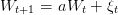
Online: computation of a control
At time t, knowing the state of the system St and the past uncertainties W0,..,Wt−1 compute a
forecast t,..,T−1 and compute Ut:
![T∑−1
Ut ∈ arg min min [ Lk (Sk,Uk, ¯wk+1) + K (ST)]
Ut∈𝕌 Ut+1,..,UT−1 k=t](subway_stations_energy_management30x.png) | (12) |
We provide a function to solve a deterministic problem knowing a scenario, the initial state and the initial time step. This function is in the file deterministic.jl.
Question 9 Use this function to solve the deterministic problem over the whole horizon with initial state x0 and initial time step 0 for each of the assessment scenarios. Why is the average cost lower than the heuristic and dynamic programming one?
We provide a function to compute a forecast at time t for the next time steps up to the rolling horizon length knowing only the state at time t.
This function is used in the MPC policy as it consists in making a forecast of the future time steps and solve a deterministic problem.
Question 10 Compute a simulation with the mpc policy for each of the assessment scenarios. Compare with the previous results.
We could improve the Model Predictive Control results. Indeed MPC performances depend significantly on the forecast quality. Here we use only information about the state of the system at time t to compute a forecast assuming all the noises are time independent. We the use the previous marginal laws to compute the forecast.
The scenario generator we provided follows the following rules:
 | (13) |
with (ξt)t∈𝕋 a sequence of gaussian white noises.
The forecast computed at each time step in the MPC strategy could be based on this model and on the last uncertainty realization. The MPC policy is not anymore a state feedback it lies in the class of mappings:
 | (14) |
We provide a MPC policy using this information
Question 11 Compute a simulation with this mpc policy for each of the assessment scenarios. Compare with the previous results.
We can build such kinds of policies in a dynamic programming framework as well.
We consider the value functions computed at section ??. During the online phase we can compute the expectation with respect to Wt by exploiting the stochastic process structure. We know here that W follows an autoregressive process (or zero during night hours). We know then that: 𝔼[g(Wt)|Wt−1 = wt−1] = 𝔼[g(awt−1 + ξt)]. Knowing the law of ξt we can therefore estimate the conditional expectation at time t.
Offline phase: computation of value functions
Ignore the dependence between the noises. We keep the same marginal laws for the random
variables. For t from T to 0 compute
![Vt(St) = mUitn∈𝕌 𝔼[Lt(St,Ut,Wt+1 ) + Vt+1 (ft(St,Ut,Wt+1 ))]](subway_stations_energy_management33x.png) | (15) |
Online: computation of a control
At each time step t, observing state St and previous uncertainty realization wt compute
Ut:
![Ut ∈ arg min 𝔼 [Lt(St,U, awt−1 + ξt) + Vt+1(ft(St,U, awt−1 + ξt))]
U ∈𝕌](subway_stations_energy_management34x.png) | (16) |
We provide a policy of this form using the value functions we generated earlier.
Question 12 Compute a simulation with this policy for each of the assessment scenarios. Compare with the previous results.
Using noises correlation information with value functions computed with time independence assumption mitgh be inefficient in practice.
When the randomness is an order 1 autoregressive process it is possible to improve the stochastic dynamic programming results by augmenting the state with 1 state variable. W follows an AR(1) process. We can then take Wt as a state variable, ξ(⋅) being the noises of the problem. We just add the following dynamic in the problem (1):
 | (17) |
W(⋅) being now a state variable and ξ(⋅) the exogenous noises process. We call the new dynamic Ft such that:
 | (18) |
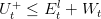
Offline phase: computation of value functions
For t from T to 0 compute
![Vt(St,Wt ) = min 𝔼[Lt(St,Wt, Ut,ξt) + Vt+1(Ft(St,Wt, Ut,ξt))]
Ut∈𝕌](subway_stations_energy_management37x.png) | (19) |
Online: computation of a control
At time t, knowing the state of the system St compute Ut:
![U ∈ arg min 𝔼[L (S ,W ,U ,ξ ) + V (F (S ,W ,U ,ξ ))]
t U∈𝕌 t t t t t t+1 t t t t t](subway_stations_energy_management38x.png) | (20) |
We define a new instantaneous cost code function, a new dynamic, a new state discretization, a new control discretization and new noises laws.
Question 13 What is the number of state variables? What is the number of control variables? What is the difference between the previous instantaneous cost and this one? Same question with the dynamics.
We build another stochastic dynamic programming model. We can generate the value functions of the problem with 2 state variables. Now the noises are truly independent.
We provide a function to compute a control online using these value functions. This is a state feedback with the augmented state. It is therefore a function of St and Wt.
Question 14 Using the ξ assessment scenarios that were generated at the beginning, corresponding to our previous assessment scenarios. Assess the policy. Display the average cost obtained.
Question 15
Compare all the methods by filling the following table. Discuss the results.