The multidimensional Black-Scholes model

LAPEYRE Bernard

February 2, 2007

Version pdf de ce document

Basket options and control variates

We consider a $d$-dimensional basket model.

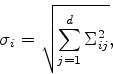
In order to correlate the assets we assume that $(W_t^1,\ldots,W_t^d,t\geq 0)$ is a vector of independent Brownian motions, that $\Sigma$ is a $d\times d$ matrix, and we define $\sigma_i$ by

$$\sigma_i = \sqrt{\sum_{j=1}^d \Sigma^2_{ij}},$$

and $\bar{W}^i$ by

$$\bar{W}^i_t = \frac{[\Sigma W_t]_i}{\sigma_i} = \frac{\sum_{j=1}^d \Sigma_{ij} W^j_t}{\sigma_i}.$$

$(\bar{W}^i_t, t\geq 0)$ is then a Brownian motion and we assume that each of the $d$ assets has a price $S^i_t$ given by a Black-Scholes model driven by the Brownian motion $\bar{W}^i$

$$\frac{d S^i_t}{S^i_t} = r dt + \sigma_i d\bar{W}^i_t, S^i_0=x_i.$$

In the numerical examples we will set $d=10$ and $x_i=100$.

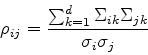
Note that $%<\bar{W}^i,\bar{W}^j>_t = \E\left(\bar{W}^i_t\bar{W}^j_t\right) = \rho_{ij} t$, where

$$\rho_{ij} = \frac {\sum_{k=1}^d \Sigma_{ik}\Sigma_{jk}} {\sigma_i\sigma_j}$$

In the numerical examples, we will assume that $\rho$ is given by $\rho^0$ where $\rho^0_{ij}=0.5$ for $i\not=j$ and $\rho^0_{ii}=1$.

1. Propose a simulation methods for the vector $(\bar{W}^1_T,\ldots,\bar{W}^d_T)$ and $(S^1_T,\ldots,S^d_T)$.
   Solution
2. We consider a basket call option on an index $I_t$ given by
   
   $$I_t = a_1 S^1_t + \cdots + a_d S^d_t.$$
   
   
   where $a_i>0$ and $\sum_{i=1}^d a_i =1$ (in numerical applications we will take $a_1=\cdots=a_d=1/d$).

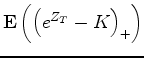
   Compute, using a Monte-Carlo method, the price of a call whose payoff is given at time $T$ by
   

   $$\left(I_T-K\right)_+,$$
   
   
   and give an estimate of the error for various values of $K$ ($K=0.8 I_0$, $K= I_0$, $K=1.2 I_0$, $K=1.5 I_0$).

   Do the same computation for an index put whose payoff is given by $(K-S_T)_+$.

   Solution
3. Prove that $\E(I_T) = I_0 \exp(rT)$. How to use $I_T$ as a control variate ? Relate this method to the call-put arbitrage relation. Test the efficiency of the method for various values of $K$.
   Solution
4. When $r$ and $\sigma$ are small, justify the approximation of $\log(I_t/I_0)$ by
   
   $$Z_T = \frac{a_1 S^1_0}{I_0} \log(S^1_t/S^1_0) + \cdots + \frac{a_d S^d_0}{I_0} \log(S^d_t/S^d_0).$$
   
   
   Prove that $Z_T$ is Gaussian with mean
   
   $$T \sum_{i=1}^d \frac{a_i S^i_0}{I_0} \left(r-\sigma_i^2/2\r... ...T \frac{1}{I_0^2} \sum_{i=1}^d \sum_{j=1}^d J_i \rho_{ij} J_j$$
   
   
   where $J_{i}= a_i S^i_0 \sigma_i$.

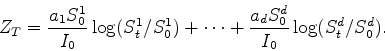
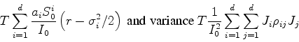
   We recall the following formula (Black-Scholes formula, exercise)
   

   $$\E\left(\left(e^Z - K\right)_+\right) = e^{\E(Z)+\frac{1}{2}\Var(Z)}N\left(d + \sqrt{\Var(Z)}\right) - KN(d)$$
   
   
   where $d=\frac{\E(Z)-\log(K)}{\sqrt{\Var(Z)}}$.

   Use this formula to give an explicit expression to $\E\left(\left(e^{Z_T} - K\right)_+\right)$ and propose a control variate technique for the computation of the call option.

   Compare this method to the standard one for different values of $K$.

   Solution

Black-Scoles model and importance sampling

We consider now the one-dimensional Black-Scholes model

$$S_t = S_0 \exp\left(\left(r-\frac{\sigma^2}{2}\right)t + \sigma W_t\right).$$

Let $S_0=100$, $\sigma=0.3$ (annual volatility) and $r=0.05$ (annual exponential interest rate).

1. We are interested in the computation of the price of a call option when $K$ is large with respect to $S_0$.

   Prove, using simulation, that the relative precision of the computation decrease when $K$ increase. Take $S_0=100$ and $K=100$, $150$, $200$, $250$. What happen when $K=400$ ?

   Solution

2. Prove that :
   
   $$\E\left(f(W_T)\right) = \E\left(e^{-\lambda W_T -\frac{\lambda^2 T}{2}}f(W_T+\lambda T)\right).$$
   
   
   Assume $S_0=100$ and $K=150$, propose a value for $\lambda$ allowing to reduce variance. Check it simulation.
   Solution