The Vasicek model is presented in Chapter ![[*]](crossref.png) .
The short rate
.
The short rate  follows the stochastic differential equation
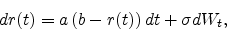 |
(1) |
where  ,
,  ,
,  are positive constants and
  is a standard
Brownian motion under
is a standard
Brownian motion under  . In computer experiments, one
can choose
. In computer experiments, one
can choose
 ,
,
 ,
,
 .
.
- Show that
 follows a Gaussian distribution with mean
 and variance

- What is the conditional distribution of
 given
given  ?
?
- Explain how to sample exactly the vector
 .
.
- Implement the suggested algorithm and plot the trajectory
for
 hour, day, week and
 .
.
We denote by  the price at time
  of a zero-coupon with
maturity date
of a zero-coupon with
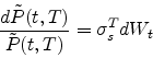
maturity date  . We assume that is a probability
under which all the discounted bond price
. We assume that is a probability
under which all the discounted bond price
are martingales.
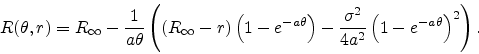
- We know (see chapter ) that
the zero coupon bonds can be written as
with :
and
 .
.
Sample the discretised trajectory price of a bond with maturity

 where day and is such that
 year.
year.
Here, we consider a call option in the Vasicek model, with maturity
 on a zero-coupon bond with maturity ,
  . We want to
implement a hedging strategy for this option.
. We want to
implement a hedging strategy for this option.
- Show, using the results of Chapter , that
where
-
Show using Proposition
that the price
 of the call option at time
, is given by
of the call option at time
, is given by
with
where  is the cumulative normal distribution function,
and
Implement this formula and plot the option price at time  as a function of the strike
  .
.
- Using Exercise of this chapter, show that
 and
and
 .
.
Implement these formulae and plot the values of  and
and
 as a function of the strike .
Give a perfect hedging portfolio for the call option using only zero
coupon bonds with maturity and zero coupon bonds with maturity
.
-
We are interested in studying discrete approximation of this
perfect hedging portfolio in which the quantity
 of
zero coupon bonds with maturity remains
constant on the interval
of
zero coupon bonds with maturity remains
constant on the interval ![$[kh,(k+1)h]$](img48.png) and equal to
and equal to  .
.
 , the quantity of zero coupon bonds with
maturity , is determined using the discrete self-financing
condition at times
, the quantity of zero coupon bonds with
maturity , is determined using the discrete self-financing
condition at times  .
.
For a given  (successively chosen to be day, week,
month) sample the residual risk of this approximated hedging
portfolio. Plot a histogram of the residual risk and study the
values of its mean and its variance when decreases to .
(successively chosen to be day, week,
month) sample the residual risk of this approximated hedging
portfolio. Plot a histogram of the residual risk and study the
values of its mean and its variance when decreases to .