 |
(1) |
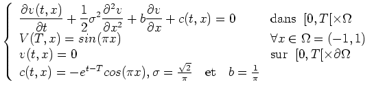
The following problem :
|
(1) |
sigma = sqrt(2)/%pi; b = 1/%pi; L=1; T=1;
hmax= sigma^2/abs(b);  // state step must be lower than hmax
pmin=ceil((2*L)/hmax)+1;
p=maxi(pmin,20);       // number of discretization points
x = linspace(-L,L,p) ;  // discretization points
x = x(2:$-1)  ;       // remove boundary points.
h=x(2)-x(1);         // state discretization step.
Question 1
Using finite difference approximations approximate the
operator
Ah such that the approximation is given by Ah*v. What are the properties
verified by Ah ? check numerically. |
sigma = sqrt(2)/%pi; b = 1/%pi; L=1; T=1;
hmax= sigma^2/abs(b);  // state step must be lower than hmax
pmin= ...
p=maxi(pmin,20);       // number of discretization points
x = linspace(-L,L,p) ;  // discretization points
x = x(2:$-1)  ;       // remove boundary points.
h=x(2)-x(1);         // state discretization step.

alpha = ..
beta =  ..
gama = ..
n= p -2 ;         // Approximate the diffusion operator
Ah= diag(beta*ones(1,n))+diag(gama*ones(1,n-1),1)+...
    diag(alpha*ones(1,n-1),-1) ;
Question 2
Using
Ah, use a Bh and Ch in such a way the the discrete version
of the continuous operators reads as
Bh and Ch. |
Question 3
Choose a time step which gives numerical stability, and solve numerically the
problem. Compare your solution with the explicit one. Compare the results with different
values of
|
theta = ...
dtmax = ... // max time step
delta = dtmax/2;
q= ... ;
delta = ...
t = linspace(0,T,q+1); // discrete time

Bmh= ...
Ch= ...

 // final condition.
deff('[y]=f(x)','y=...')
fh = feval( x' , f);

// instantaneous cost.

deff('[y]=g(x,t)','...') ;
c=feval(x,t,g);         // la fonction \(c(t,x)\) }

v=zeros(n,q+1);
v(:,q+1)=fh ;    // initialisation de \(v(x,T) \)}
for i=(q:-1:1) ,
  v(:,i) = ...
end

plot3d(x/maxi(x),t,v/maxi(abs(v)),35,45,"X@T@V");

// compare with explicit solution.

deff('[y]=Vref(x,t)','y=exp(t-T)*sin(%pi*x)');
vref=feval(x,t,Vref);
Er=maxi(abs(vref-v))
Question 4
Note that you can use scilab to solve the linear system which gives
|
We will here solve by finite differences the problem :
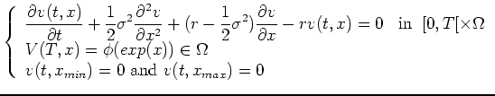 |
(2) |
which is obtained when solving the black and scholes equation in the ![]() version.
version.
Question 5
Using finite difference approximations approximate the diffusion
operator by building a matrix
Ah such that the approximation is given by
Ah*v. What are the properties verified by Ah ? check numerically.
The discretisation will take care of the fact that we use null dirichlet boundary
conditions. |
r = 0.05; sigma = 0.3; // constants
hmax=...              // max value for state step size
h=..                  // selected step size
L=5; // x in [-L,L]   // we discretize x in [-L,L]
pmin= ..              // min number of points
p=maxi(p,100);
h = L/p;
x = ...              // discrete points

alpha = ...
beta =  ...
gama =  ...
n= 2*p+1;
Ah= diag(beta*ones(1,n))+diag(gama*ones(1,n-1),1)+ diag(alpha*ones(1,n-1),-1) ;
Question 6
Using
Ah, use a S and R in such a way the the discrete version
of the continuous operators reads as
Bh and Ch. |
T=1;  // horizon
theta = 1/2; // theta used in the theta schema
dtmax = ... // statbility condition

delta = dtmax/2;
q= ceil((T/delta));
q=maxi(q,50);
delta = T/q;
t = T*(0:q)/q; // discrete times

S= ...
R= ...
Question 7
Solve the discrete parabolic problem
|
K= 40;

deff('[y]=f(x)','...')  // a call or a put
fh = feval( x' , f); // the value of v at time T
v=zeros(n,q+1);
v(:,q+1)=...  // final condition

// iteration

for i=(q:-1:1) ,
   v(:,i) =...
end

plot3d(x/maxi(x),t,v/maxi(abs(v)))
Question 8
Plot the solution when x is in the range
|
xbasc();
i1=...
i2=...
xn=x(i1:i2)';
for i=1:q+1; plot2d(xn,v(i1:i2,i));end
Question 9
We can compare the numerical solution with an explicit one
(since
cdfnor to evaluate
the cumulative distribution function of the normal distribution and its inverse. |
S0=K;
d1=(1/(sigma*sqrt(T)))*(log(S0/K)+(r+sigma**2/2)*T);
d2=d1-sigma*sqrt(T);
call_price=S0*cdfnor("PQ",d1,0,1)-K*exp(-r*T)*cdfnor("PQ",d2,0,1);
put_price=-(S0-K*exp(-r*T))+(S0*cdfnor("PQ",d1,0,1)-K*exp(-r*T)*cdfnor("PQ",d2,0,1));

p = ...

// compare p with the call price or the put_price.
p -call_price  ...