Abstract
In this practical work, you will play the role of a dam manager. You will try to maximize the mean intertemporal payoff obtained by selling hydropower produced by water releases, when the water inflows (rain, snowmelt, outflows from upper dams) are supposed to be random and the energy prices deterministic. You will propose different water turbinated policies and you will compute their expected payoff. Then, you will compute the optimal payoff and display an optimal policy. At last, you will consider different variations around this problem: highlighting the information structure influence by comparing the “decision-hazard” and the “hazard-decision” settings, evaluating a “fair final value of the water” or testing robustness with respect to inflow probability distribution.
We consider a dam manager intending to maximize the intertemporal payoff obtained by selling power produced by water releases, when the water inflows (rain, snowmelt, outflows from upper dams) are random and the energy prices are supposed to be deterministic.
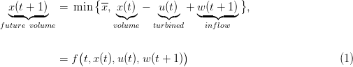
We model the dynamics of the water volume in a dam by a function f defined as follows1
where
 | (2) |
The dam manager is supposed to make a decision at each t ∈ 𝕋, here turbinating u(t) at the beginning of the period [t,t + 1[, before knowing the water inflow w(t + 1): such a setup is called decision-hazard setting. We add the following constraint on the turbinated water:
 | (3) |
Constraint (3) ensures u(t) is feasible, that is, such that the dam volume remains greater or equal to its minimum value x (remember that any inflow w(t) is nonnegative).
The manager problem is one of payoff maximization. At each time t, the turbinated water u(t) produces electricity which is sold on markets at a price p(t). The associated financial income is modeled by a linear function L(t,u) = p(t)u, leading to the instantaneous payoff
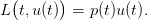 | (4) |
Moreover, the volume x(tf) remaining in the dam at the horizon tf is valued (this is the so-called final value of water) using a quadratic function K, leading to the final payoff
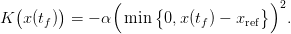 | (5) |
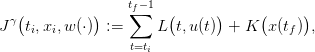
Here, α is a coefficient and xref is a given reference volume for the dam at horizon tf. The final payoff is negative if and only if x(tf) < xref. From ti to tf, the payoffs sum up to
 | (6) |
The sequence of prices  p(ti),…,p(tf − 1)
 is supposed to be deterministic, hence known in advance
at initial time ti where the optimization problem is posed.
is supposed to be deterministic, hence known in advance
at initial time ti where the optimization problem is posed.
A water inflow scenario is a sequence of inflows in the dam from time ti up to tf − 1
 | (7) |
We model water inflow scenarios using a sequence of random variables with a known joint probability distribution ℙ such that
 w(ti),…,w(tf − 1)
 are independent,
 | (8) |
Notice that the random variables  w(ti),…,w(tf − 1)
 are independent, but that they are not
identically distributed. Independence is a key assumption to obtain the dynamic programming
equation (18) with state x.
are independent, but that they are not
identically distributed. Independence is a key assumption to obtain the dynamic programming
equation (18) with state x.
Time. We consider a montly management (the interval [t,t + 1[ represents one month) over one year, so that
 | (9) |
State and control. Concerning the dam volume and the turbinated water, we consider the following bounds:
 | (10) |
We assume that the dam volume is discretized using a stepsize δx = 2 hm3, whereas the stepsize used for discretizing the control is δu = 8 hm3 (multiple of δx). Accordingly, the sets containing the possible values of the state and the control are
 |
The water volume in the dam at time ti is known and equal to xi = 40 hm3, and the reference volume used to define the final payoff K in (5) is xref = 40 hm3.
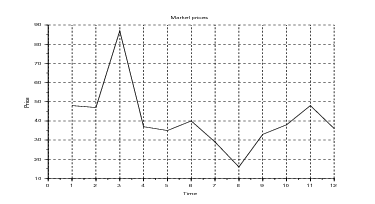
Prices scenario.
The price scenario  p(ti),…,p(tf − 1)
 , known in advance, is shown in Figure 1.
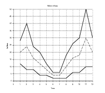
Water inflow scenarios. At each time t, the range 𝕎(t) of the water inflow w(t) is obtained by discretizing an interval centered around a given mean value (see Figure 2). Each interval is discretized using a stepsize δw = 2 hm3 (multiple of δx). Consider for example time t = 1: the minimum (resp. maximum) inflow value is w(1) = 12 hm3 (resp. w(1) = 28 hm3), so that the finite support 𝕎(1) of the (uniform) probability distribution associated with the random variable w(1) is
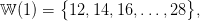 |
the probability weight of each element w ∈ 𝕎(1) being 1∕9.
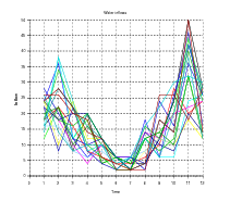
Knowing the probability distribution, it is easy to draw water inflow scenarios since we assumed that the random variables w(t) are independent.
Scilab code. The following Scilab code contains the data and macros corresponding to the numerical example described in §1.4.
Question 1
In order to simulate (and then optimize) the dam behavior, we need to have the Scilab macros computing the dynamics (1) and the payoffs (4) and (5).
Question 2 [2] Copy the above Scilab code at the end of the file DamManagement.sce and check that it corresponds to the expressions (1)–(4)–(5). Notice that these macros are written in such a way that they may be fed either with scalar values or with vector values. This feature will be be used for efficiently simulating a bunch of inflow scenarios (see Question 3).
An admissible policy γ : 𝕋 × 𝕏 → 𝕌 assigns a turbinated water amount u = γ(t,x) ∈ 𝕌 to any time t ∈ 𝕋 and to any dam volume x ∈ 𝕏, while respecting constraint (3), that ias,
 |
Hence, by (2), we obtain that
 |
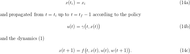
Given an admissible policy γ and given an inflow scenario
 | (11) |
we are able to build a dam volume trajectory
 | (12) |
and a turbinated water trajectory
 | (13) |
produced by the “closed-loop” dynamics initialized at the initial time ti by
We also obtain the payoff associated to the inflow scenario w(⋅)
 | (15) |
where x(⋅) and u(⋅) are given by (14c). The expected payoff associated with the policy γ is
 | (16) |
where the expectation 𝔼 is taken with respect to the product probability ℙ,
whose marginals are given by (8). The true expected value (16) is difficult to
compute,3
and we evaluate it by the Monte Carlo method using Ns inflow scenarios  w1(⋅),…,wNs(⋅)
 :
:
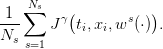 | (17) |
By the law of large numbers, the mean payoff (17) is a “good” approximation of the expected payoff(16) if the number of scenarios is “large enough”.
We propose the following Scilab code in order to evaluate the mean payoff associated to a policy given by the Scilab macro policy.
Question 3
In order to test the Scilab macro simulation given above, consider the following code.
Question 4
We now want to design new policies, writing Scilab macros following the model given by the macro below:
Question 5
and evaluate them thanks to the scenario based simulator.
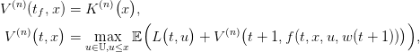
In order to compute the optimal turbinated water policy, we provide the stochastic dynamic programming (or Bellman) equation associated with the problem of maximizing the expected payoff (16), as well as the corresponding Scilab code.
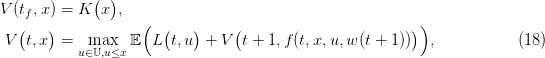
Since the water inflows w(t) are supposed to be independent random variables, Dynamic Programming applies and the equation associated with the problem of maximizing the expected payoff (16) writes
for t varying from tf − 1 to ti. The expectation 𝔼 is taken with respect to the marginal probability distribution ℙw(t+1) given by (8), that is,
 |
A difficulty when programming the Bellman equation is that we need to manipulate both the values (t,x) of the time and of the state, and the associated indices (t,i) in the table storing the values of the function V (t,x). In our application, the treatment of index t is obvious because t ∈ 𝕋 = {ti,ti + 1,…,tf}, but we need a tool performing the conversion for the volume. The following Scilab macro state_index returns the index i associated to an element x in the finite set 𝕏 containing the possible values of the dam volume.
We provide the following code in order to compute the Bellman function.
Question 7
Consider the following Scilab macro.
Question 8
Here we assume that the values of optimal control have not be stored in the table Ubell, so that the only outcome of the macro sdp_solve is the table Vbell (Bellman values).
Question 9 [2] Provide a method and the corresponding code to compute the optimal value of the control at time t for a given dam volume x(t) using only the values stored in the table Vbell at time t + 1.
Hint: the optimal control at (t,x(t)) is the arg max of the following optimization problem:
 | (19) |
Be careful that your code must accept a vector of volumes as input.
In this section, we propose several developments and extensions for the dam management problem.
In the hazard-decision framework, the dam manager is supposed to make a decision, here turbining u(t) at the beginning of the period [t,t + 1[, knowing the water inflow w(t + 1) in advance.
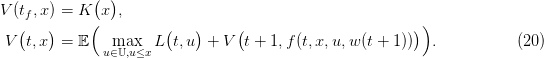
The Bellman equation is now
Once the value function V (t,x) evaluated and stored for all time t and state x, the optimal control at time t starting from state x and observing the water inflow w is the arg max of
 | (21) |
which leads to an optimal policy depending on the triplet (t,x,w).
Question 10
Till now, the gain in leaving water in the dam at the end of the time horizon was arbitrarily fixed.
Now, we provide a procedure to estimate a “ fair final value of water”, that is, a function x K(x)
as in (5).
K(x)
as in (5).
The intuition behind the procedure is that the final value of water is the value that a manager would put on the dam, were he to run it from the date tf + 1 to infinity. The final value of water is the solution of an infinite horizon maximization problem. The procedure below mimicks an algorithm to find a fixed point by iterations.
First, we start with a zero final payoff function  and obtain, by backward
induction, the Bellman function
and obtain, by backward
induction, the Bellman function  at initial time ti. Up to a translation — to account for
the fact that an empty dam has zero final value of water — we identify the function
at initial time ti. Up to a translation — to account for
the fact that an empty dam has zero final value of water — we identify the function
 with the new final value of water
  . Proceeding along, we expect
that this loop converges towards a function x
. Proceeding along, we expect
that this loop converges towards a function x K(∞)(x) which is a good candidate for the final
value of water.
K(∞)(x) which is a good candidate for the final
value of water.
We design a loop for n = 1,…,N, starting with a zero final value of water
 |
then solving the backward Bellman equation
and then closing the loop by choosing the new final value of water
 | (22) |
as the Bellman function at the initial time ti after a shift, so that K(n+1)(x) = 0.
Question 11 Implement the iterative procedure described above, and compute and plot the “fair final value of water” in the dam.
An interesting point, which occurs in practical problems, is the following. In the case where the
random variables  w(ti),…,w(tf − 1)
 are correlated in time, it is always possible to obtain the
marginal probability laws ℙw(t) of each w(t) and then compute the Bellman function as
in §3. We thus obtain a feedback policy that would be optimal if the random inflow
variables were uncorrelated. The loss of optimality may be evaluated by simulating the
feedback policy along scenarios drawn using the “true” probability law ℙ of the process
are correlated in time, it is always possible to obtain the
marginal probability laws ℙw(t) of each w(t) and then compute the Bellman function as
in §3. We thus obtain a feedback policy that would be optimal if the random inflow
variables were uncorrelated. The loss of optimality may be evaluated by simulating the
feedback policy along scenarios drawn using the “true” probability law ℙ of the process
 w(ti),…,w(tf − 1)
 .
.
Question 12