Optimal Resources Allocation in Ecology:
to Grow or to Reproduce? (I)
The Constant Environment Case

Michel de lara¹
(last modiﬁcation date: October 10, 2017)

Version pdf de ce document
Version sans bandeaux

1 Life History Patterns Exhibit Large Variety
2 The Basic Model of an Annual Plant Growth by Amir and Cohen (1990)
3 Optimal Allocation in Constant Environnement (Theory)
4 Comparison of Strategies in Constant Environment (PW Scilab)
5 Numerical Evaluation of Optimal Strategies in Constant Environment (PW Scilab)
6 Scilab Code

1 Life History Patterns Exhibit Large Variety
2 The Basic Model of an Annual Plant Growth by Amir and Cohen (1990)
3 Optimal Allocation in Constant Environnement (Theory)
3.1 Optimisation model in constant environnement
3.2 Resolution by dynamic programming
4 Comparison of Strategies in Constant Environment (PW Scilab)
4.1 Dynamics of the plant
4.2 Costs functions
4.3 Comparison between strategies
5 Numerical Evaluation of Optimal Strategies in Constant Environment (PW Scilab)
5.1 Parameters
5.2 State, control and cost discretization
5.3 Discretization of the dynamics. Transition matrices
5.4 Numerical resolution by dynamic programming
6 Scilab Code

1 Life History Patterns Exhibit Large Variety

“ Herbs often ﬂower in their ﬁrst year and then die, roots and all, after setting seed. Plants that ﬂower once and then die are monocarpic.

Many monocarps are annual but a few species have long lives. Bamboos are grasses but they grow to unusually large size. One Japanese species, Phyllostachys bambusoides, waits 120 years to ﬂower (Janzen, 1976).

Most trees ﬂower repeatedly. However, Foster (1977) has characterized Tachigalia versicolor as a ’suicidal neotropical tree’. After reaching heights of 30-40 m, it ﬂowers once and then dies. ”

(Cited from Mark Kot, Elements of Mathematical Ecology, Cambridge University Press, 2001)

Mammals and other organisms present determinate growth: they stop growth when they become mature and start to reproduce. But many animals and plants, such as ﬁshes, snakes, clams, etc. experience indeterminate growth: they life-history shows trade-oﬀs between growth and reproductiwe havelong their lifetime.

2 The Basic Model of an Annual Plant Growth by Amir and Cohen (1990)

The model of single plant growth of [1] depends on three factors:

a (deterministic) integer T, the maximum length of the growing period (number of days, weeks or months in one year, for instance);
an integer random variable 𝜃, interpreted either as an individual lifetime length or as a growing season length;
a growth function f : ℝ₊ × ℝ₊ → ℝ₊: if, at the beginning of time interval [t,t + 1[, x is the vegetative biomass of the plant and e is the state of the environment, then f(x,e) ≥ 0 is the maximum total biomass (vegetative and reproductive) which may be generated by the plant during [t,t + 1[ (depends on roots, leaves, environmental factors, etc.).

The dynamics is a follows.

At the beginning of each time interval [t,t + 1[, the plant
- is characterized by its vegetative biomass x_t ∈ [0, +∞[ (state);
- is able to mobilize resource to generate the total biomass f(x_t,e_t);
- allocates biomass f(x_t,e_t) − u_t as reproductive biomass in the interval [t,t + 1[, where 0 ≤ u_t ≤ f(x_t,e_t).
At the end of each time interval [t,t + 1[,
- the annual reproductive yield is S_t+1 = ∑ _s=0^t[f(x_s,e_s)−u_s] = S_t+[f(x_t,e_t)−u_t];
- the vegetative biomass is x_t+1 = u_t.

In the ﬁrst part of the paper, Amir and Cohen consider one source of stochasticity, namely 𝜃, before introducing also the environment e as random. The dynamics above is randomly aborted at 𝜃 giving the annual reproductive yield per plant:

∑𝜃 S𝜃 := [f(xt,et) − ut]. t=0

(1)

Note that the constraint 0 ≤ u_t ≤ f(x_t,e_t) implies two biological as:

u_t = 0 is a possible decision, meaning that the plant may “decide” to die;
u_t ≤ x_t is a possible decision, meaning that the plant may transfer a fraction of its vegetative biomass to reproductive biomass, by reducing its present size (for some organisms, as ﬁshes, for which size may not decrease with time, we shall rather impose x_t ≤ u_t).

3 Optimal Allocation in Constant Environnement (Theory)

3.1 Optimisation model in constant environnement

Dynamics

Consider an annual plant which grows and reproduces according to the following dynamics

yt + xt+1 = f(xt), t = 0,...,T − 1

(2)

where

T is the maximum length of the growing period (number of days, weeks or months in one year, for instance), with T < +∞;
x_t is the vegetative biomass at the beginning of period [t,t + 1[;
y_t is the reproductive biomass produced during period [t,t + 1[.

Here are the general assumptions on the growth function :

f is C² on ]0, +∞[ [technical assumption];
f(0) = 0 and f(x) > 0 for x > 0 [the growth function measures a biomass];
f is nondecreasing: f′≥ 0 [the bigger you are, the more biomass you generate];
f is concave: f′′≤ 0 [the bigger you are, the lower your rate of biomass generation].

Random mortality

Let us assume that the plant lives for a random number 𝜃 of periods, with the random variable 𝜃 following a geometric law with parameter β, survival probability :

t ∀t ∈ ℕ, ℙ(𝜃 ≥ t) = β .

(3)

We assume that death occurs at the end of a period. Thus, on the event {𝜃 = t}, the plant dies at the end of period [t,t + 1[, leaving reproductive biomass f(x_t) = f(x_𝜃) and vegetative biomass x_t+1 = x_𝜃+1 = 0.

Decisions and strategies

Consider a plant with vegetative biomass x_t at the beginning of period [t,t + 1[. It will generate total biomass f(x_t) at the end of the period. This biomass will be split between reproductive biomass y_t and future vegetative biomass x_t+1. What we call here a “decision” for the plant corresponds to the choice of an allocation between reproductive biomass and future vegetative biomass.

Let us introduce the decision variable

ut = xt+1 ∈ [0,f(xt)].

(4)

We deﬁne a strategy for the plant as a sequence of decisions

(u ,u ,...,u ) with 0 ≤ u ≤ f(x ),...,0 ≤ u ≤ f(x ). 0 1 T −1 0 0 T −1 T− 1

(5)

Mathematically speaking, a strategy is a mapping

u() : {0, ...,T − 1} × ℝ+ → ℝ+

(6)

such that u(t,x) ∈ [0,f(x)].

Criterion

We shall say that a strategy is optimal if it maximizes the mathematical expectation of the ﬁtness (individual contribution to future generations):

(T−∑ 1)∧𝜃 J (u(.)) = 𝔼 ( [f(xt) − ut]), u(.) = (u0,u1,...,uT− 1). t=0

(7)

Here, the ﬁtness is deﬁned as the cumulated reproductive biomass at the end of the growing season (the annual reproductive yield for an annual plant).

An optimal trajectory is any sequence (x₀,...,x_T) generated by

xt+1 = f(xt) − ut, ut = u♯(t,xt), t = 0,...,T − 1

(8)

where u^♯ is an optimal strategy.

Why should natural selection favor such optimal strategies?

Consider various plants with various strategies. At the end of the growing season, those plants with an optimal strategy should, in the mean (because a mathematical expectation is maximized), be relatively more numerous than the others. Season after season, their relative number would grow.

When variability is between individuals within the same season (independent lifetimes) and when the populations are suﬃciently large, the law of large numbers applies and this justiﬁes the expected value of the annual reproductive yield as appropriate measure of ﬁtness. Other approaches deﬁne an optimal strategy as one not susceptible to be invadable by a mutant.

A deterministic optimization problem

Here, the expectatiwe above is with respect to the only source of randomness, namely 𝜃.

Question 1 Show that

(T−∑1)∧𝜃 T∑−1 J(u (.)) = 𝔼( [f (xt) − ut]) = βt[f(xt) − ut], t=0 t=0

(9)

Thus, identifying optimal strategies amounts to solving

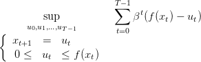
T∑ −1 sup βt(f(x ) − u ) u0,u1,...,uT−1 t t { t=0 xt+1 = ut 0 ≤ ut ≤ f (xt)

(10)

This is a deterministic dynamic optimization problem with additive criterion characterized by

instantaneous cost l(t,x,u) = β^t(f(x) − u),
zero ﬁnal cost (there is no term with x_T in the criterion).

3.2 Resolution by dynamic programming

The dynamic programming equation (dpe) is

V (x,t) = sup (βt(f(x ) − u) + V (u,t + 1)) with V (x, T) = 0. 0≤u≤f(x)

(11)

Denoting

-- V (x,t) :=-1-V(x, t) βt

(12)

the dpe may equivalently be written as

-- -- -- V (x,t) = sup (f (x) − u + βV (u,t + 1 )) with V(x, T) = 0. 0≤u≤f(x)

(13)

Optimal strategies u^♯ are solution of

-- u♯(t,x) ∈ 𝒰♯(t,x) := arg max (f (x) − u + βV (u,t + 1)). 0≤u≤f(x)

(14)

Question 2 Show that V (x,T − 1) = f(x) and that the last optimal decision u^♯(T − 1,x) consists in allocating all available biomass at the end of period [T − 1,T[ into reproductive biomass, and thus die at T.

There is no gain in terms of oﬀspring to keep vegetative biomass at the end of the last period.

Linear growth function

Let us suppose here that

f (x) = rx.

(15)

Question 3

Assume that βr ≤ 1. Show that, for t = 0,...,T − 1, V (t,x) = rx and 𝒰_t^♯(t,x) = {0}. Describe the proﬁle of an optimal trajectory.
Assume that βr > 1, Show that, for t = 0,...,T − 1, V (t,x) = (βr)^T−t−1rx and 𝒰_t^♯(t,x) = {rx}. Describe the proﬁle of an optimal trajectory.

Strictly concave growth function with low slope

Let us suppose here that

′ 1- ∀x ≥ 0, f (x) ≤ β.

(16)

Question 4 Show that, for t = 0,...,T − 1, V (t,x) = f(x) and 𝒰_t^♯(t,x) = {0}. Describe the proﬁle of an optimal trajectory.

Marginalist economic interpretation: whatever the plant size, the expected marginal gain in future biomass (βf′(x)) is always less than the direct gain in oﬀspring (+1 by renouncing to growing by one unit).

Strictly concave growth function with high slope

Let us suppose here that

1 ∀x ≥ 0, f ′(x) > -. β

(17)

Question 5 Show that, for t = 0,...,T − 1, 𝒰_t^♯(t,x) = {f(x)}. Describe the proﬁle of an optimal trajectory.

Marginalist economic interpretation: whatever the plant size, the expected marginal gain in future biomass (βf′(x)) is always greater than the direct gain in oﬀspring (+1). An example is given by the ’suicidal neotropical tree’ Tachigalia versicolor.

Strictly concave growth function with moderate slope

Let us suppose here that

′ ∃x+ > 0, βf (x+ ) = 1.

(18)

Together with the target x₊, let us deﬁne the threshold

x − := f −1(x+).

(19)

Thus, the function u− u + βV (u,t) is nondecreasing up to x⁺, then nonincreasing.

Question 6 Show that an optimal decision rule at period T − 2 is

if the vegetative biomass at the beginning of period [T−2,T−1[ is less than the threshold x₋, allocate total biomass into vegetative biomass;
if the vegetative biomass at the beginning of period [T − 2,T − 1[ is greater than the threshold x₋, allocate part of total biomass to obtain vegetative biomass x₊; the rest f(x) − x⁺ ≥ 0 is allocated to reproductive biomass.

Question 7 Show that

V (x,T − 2) is continuous and continuously diﬀerentiable at x = x₋, and that β(x₊,T − 2) = 1;
V (x,T − 2) is continuously diﬀerentiable and that (x,T − 2) is decreasing.

Deduce from this that optimal decision rules at periods T − 2 and T − 3 coincide.

Going backward, one may show that, for all t = 0,...,T − 2, growing without reproducing when vegetative biomass is under threshold x⁻ and growing up to the target x⁺ if not is the optimal strategy (except at the last season).

Marginalist economic interpretation: at the target x⁺, the expected marginal gain in future biomass (βf′(x⁺)) is equal to the direct gain in oﬀspring (+1). Examples are given by mammals (including whales and humans).

4 Comparison of Strategies in Constant Environment (PW Scilab)

Let us take

f(x,r) = rxγ with 0 < γ ≤ 1.

(20)

To facilitate computer programming, the control is no longer u_t ∈ [0,f(x_t)], but

ut vt :=------∈ [0,1] (vt = 0 if f(xt) = 0). f (xt)

(21)

Thus, this control v belongs to a ﬁxed interval [0, 1], contrarily to u ∈ [0,f(x)].

We incorporate the random time 𝜃 directly in a stochastic dynamics as follows

xt+1 = F (xt,vt,st), t = 0,...,T − 1, vt ∈ [0,1], st ∈ {0, 1}.

(22)

Here, s_t = 0 means that the plant dies at the end of period [t,t + 1[, while s_t = 1 corresponds to survival. The sequence s₀,...,s_T−1 is i.i.d. with binomial distribution ℙ(s_t = 1) = β.

4.1 Dynamics of the plant

Open a ﬁle plantI1.sci and write a Scilab function dyn_plant representing the growth function, depending on the state x (the value of the parameter r will be given later).

  function b=dyn_plant(x)
    // b = total biomass generated by the plant in one period
    //x = vegetative biomass
    b=r*x^{power}
  endfunction

In the ﬁle plantI1.sci, write the fonction dyn_plant_control.

  function b=dyn_plant_control(x,v,s)
    // Growth function, with control v and random term s
    // b = future vegetative biomass
    // x = vegetative biomass
    // v = fraction allocated to growth (control)
    // s = survival factor (s=1 survival, s=0 death)
    // if s=0, x transits towards 0
    // if s=1, x transits towards v*dyn_plant(x)
    if v < 0 | v > 1 then
      b='ERROR : control beyond bounds'
    else
      if s==0 then
        b=0
        //transition towards 0 if the survival factor is zero
      else
        b=v*dyn_plant(x)
      end
    end
    // the formula b=s.*v.*dyn_plant(x) has a problem?
  endfunction

4.2 Costs functions

In the ﬁle plantI1.sci, write the following instantaneous and ﬁnal costs functions.

  // ateb instead of beta, since beta may be a predefined Scilab macro

  function cost=offspring(state,control,time)
    cost=(1-control)*ateb^{time}*dyn_plant(state);
  endfunction

  function cost=final_cost_zero(state,time)
    cost=0;
  endfunction

4.3 Comparison between strategies

Examples of strategies

In the ﬁle plantI1.sci, write the following Scilab macros:

strategie_D (D for die) representing the strategy “to reproduce and to die”: the output of strategie_M is 0;
strategie_R (R for random) representing a uniform random decision: the output of strategie_R is a random real in [0, 1];
strategie_G (G for growth) representing the strategy “growing without reproducing except at the last decision period”: the output of strategie_G is either 0 (to reproduce and die) or 1 (to grow without reproducing).

  function v=strategy_D(t,x)
    v=0
  endfunction

  function v=strategy_R(t,x)
    v=rand()
  endfunction

  function v=strategy_G(t,x)
    if t < T then
      // t=1:T corresponds to t=0,...,T-1
      v=1
    else
      v=0
    end
  endfunction

Scilab functions for trajectory evaluation

In the ﬁle plantI1.sci, write the following Scilab function traj_feedback with arguments

an initial state,
a Scilab function controlled_dynamics (similar to dyn_plant_control),
a Scilab function feedback (similar to strategy_X),
a random vector (two-dimensional: survival alea and resources alea; this latter alea is of no use at this stage)

and with outputs the corresponding state and control trajectories after feedback.

  function [x,v]=traj_feedback(initial_state,controlled_dynamics,feedback,alea)
    // initial_state
    // controlled_dynamics(x,v,s) : returns a state
    // feedback(t,x) : returns a control
    // alea : sequence of 0 or 1, with length horizon
    // x : state trajectory
    // v : control trajectory
    horizon=size(alea,2);
    x=initial_state
    v=[]
    for t=1:horizon do
      // t=0,...,T-1
      v=[v,feedback(x($),t)]
      // x($) is the last value of vector x
      // v has dimension horizon=T
      x=[x,controlled_dynamics(x($),v($),alea(t))]
      // x has dimension 1+horizon=1+T
    end
  endfunction

In the ﬁle plantI1.sci, write the following Scilab function total_cost with arguments

trajectory, a state trajectory, that is a vector with dimension (1,T + 1)
control, a control trajectory, that is a vector with dimension (1,T)
a Scilab function inst_cost,
a Scilab function fin_cost,

and with output the value of the additive criterion along state and control trajectories.

  function cost=total_cost(trajectory,control,inst_cost,final_cost)
    // trajectory is a vector of dimension 1+horizon,
    // control is a vector of control of dimension horizon
    // inst_cost(state,control,time) is a function
    // final_cost(state,time) is a function
    // cost is a vector of dimension 1+horizon, comprising the sequence of
    // cumulated sums of instantaneous cost (and of final cost)

    horizon=prod(size(control))

    if 1+horizon <> prod(size(trajectory)) then
      cost='ERROR : dim(trajectory) different from 1+dim(control)'
    else
      cost=[]
      for t=1:horizon do
        // i.e. t=0,...,T-1
        cost=[cost,cost($)+inst_cost(trajectory(t),control(t),t)]
        // cumulated sums of instantaneous cost
      end
      cost=[cost,cost($)+final_cost(trajectory(1+horizon),1+horizon)]
    end
  endfunction

Linear growth function

Open a ﬁle plantI1.sce. In this ﬁle, we will ask to load the macros in the ﬁle plantI1.sci and we will change the values of the following parameters.

  // exec('plantI1.sce')
  // parameters
  power=1;//  gamma
  ateb=0.9,// survival probability
  r=1.2;
  T=10;
  x0=1;
  // ATTENTION. The control is mathematically indexed by t=0,...,T-1.
  // However, it is indexed by 1:T=1:horizon in Scilab
  // The state is indexed by 1:(T+1)=1:(1+horizon) in Scilab

Question 8 Compute state and control trajectories in closed loop with the diﬀerent strategies strategy_X. Use for this Scilab function traj_feedback.

Compute corresponding ﬁtness. Use for this Scilab function total_cost.

Draw state, control and ﬁtness trajectories thanks to Scilab macro plot2d2.

Write these instructions in ﬁle plantI1.sce, and execute them by exec(’plantI1.sce’).

  exec('plantI1.sci');
  strategy=list();
  strategy(1)=strategy_D;
  strategy(2)=strategy_R;
  strategy(3)=strategy_G;

  correspondance=list();
  correspondance(1)=string("death");
  correspondance(2)=string("random");
  correspondance(3)=string("growth");

  // In what follows, we adopt the terminology
  // of the arguments of function traj_feedback
  initial_state=1;
  dynamics=dyn_plant_control;
  alea=ceil(ateb-rand(1,T));
  // T independsent realizations of a binomial law B(ateb,1)
  inst_cost=offspring;
  final_cost=final_cost_zero;

  for i=1:3 do
    [b,v]=traj_feedback(initial_state,dynamics,strategy(i),alea);
    f=total_cost(b,v,inst_cost,final_cost);

    xset("window",3*(i-1));xbasc();plot2d2(1:T+1,f,rect = [0,0,T+2,max(f)+1]);
    xtitle("strategy "+correspondance(i)+" : fitness");

    xset("window",3*(i-1)+1);xbasc();plot2d2(1:T,v,rect = [0,0,T+1,max(v)+1]);
    xtitle("strategy "+correspondance(i)+" : control");

    xset("window",3*(i-1)+2);xbasc();plot2d2(1:T+1,b,rect = [0,0,T+2,max(b)+1]);
    xtitle("strategy "+correspondance(i)+" : state");

    printf("the total fitness for strategy "+correspondance(i)+" is : %"+" f\n",f($))

    halt();
    xdel((3*(i-1)):(3*(i-1)+2));
    // deletes the windows
  end

Question 9 Compare total ﬁtness for the diﬀerent strategies.

Strictly concave growth function with moderate slope

Question 10 Give analytical expressions of x₊ and x₋ deﬁned at equations (18) and (19). Write in Scilab the corresponding formulas xp and xm.

  // parameters
  power=0.5;
  xp=(ateb*r*power)^{1/(1-power)};
  xm=(xp/r)^{1/power};

Question 11 In ﬁle plantI1.sci, write a Scilab function strategy_O ( _O for optimal), with arguments a state x and a time t, and with output following feedback rule:

if the vegetative biomass is less than x₋, do no reproduce;
if the vegetative biomass is greater than or equal to x₋, then the future vegetative biomass will be x₊.

Check, with the above theoretical results, that this strategy is optimal.

  function v=strategy_O(t,x)
    if x < xm then
      v=1
    else
      v=xp/dyn_plant(x)
    end
  endfunction

Question 12 Do the same questions as above with the following strategy.

strategy(4)=strategy_O;
correspondance(4)=string("optimal");

Question 13 What do you observe when γ varies in [0, 1]?

  P=0.1:0.2:0.9;
  for j=1:prod(size(P)) do
    power=P(j);
    xp=(ateb*r*power)^{1/(1-power)};
    xm=(xp/r)^{1/power};
    x0=xm/10;
    // initial biomass less than threshold xm
    printf("gamma=%"+" f\n",P(j));
    for i=1:4 do
      [y,v]=traj_feedback(x0,dynamics,strategy(i),alea);
      f=total_cost(y,v,inst_cost,final_cost);
      printf("the total fitness for strategy "+correspondance(i)+" is : %"+" f\n",f($))
    end
  end

5 Numerical Evaluation of Optimal Strategies in Constant Environment (PW Scilab)

We take

0 < γ < 1.

(23)

5.1 Parameters

Copy the following parameters in a ﬁle plantI2.sce.

  // exec('plantI2.sce')
  T=10;
  ateb=0.9;
  r=1.2;
  power=0.5;

5.2 State, control and cost discretization

Copy the following code in ﬁle plantI2.sce. It provides the state and control discretizations, as well as instantaneous cost and ﬁnal cost. See Programmation dynamique, macros generales.

  state=[0:(xm/6):(1.2*xp)];
  control=0:0.05:1;

  offspring=list();
  discount=cumprod([1,ateb*ones(1,T-1)]);
  for l=1:prod(size(control)) do
    offspring(l)=(1-control(l))*(r*(state')^{power})*discount;
    // offspring(l) is a matrix
  end

  final_cost_zero=zeros(state');

Note that Scilab functions deﬁned in Section 4 are now redeﬁned.

5.3 Discretization of the dynamics. Transition matrices

Get the Scilab functions predec_succes, egal and discretisation from Programmation dynamique, macros generales and copy them in the ﬁle plantI2.sci, as well as the following function.

  function b=dyn_plant_control(x,v)
    //b = total biomasse
    //x = vegetative biomass
    //v = control
    b=v*r*x^{power}
  endfunction

Copy the following code in ﬁle plantI2.sce.

  exec('plantI2.sci')

  controlled_dynamics=dyn_plant_control;

  transition_matrix=discretisation(state,control,controlled_dynamics);

Question 14 Check that the list of matrices matrix_transition indeed consists of transition matrices, that is with nonnegative coeﬃcients summing to 1 on each row.

  cardinal_control=size(transition_matrix);
  for l=1:cardinal_control do
    sum(transition_matrix(l),"c")'
    mini(transition_matrix(l))
    maxi(transition_matrix(l))
    halt();
  end

5.4 Numerical resolution by dynamic programming

Get the Scilab functions Bell_stoch and trajopt from Programmation dynamique, macros generales and copy them in ﬁle plantI2.sci

Copy the following code in ﬁle plantI2.sce.

  instant_cost=offspring;
  final_cost=final_cost_zero;

  [value,feedback]=Bell_stoch(transition_matrix,instant_cost,final_cost,1);
  // solves the dynamic programming equation

  initial_state=grand(1,1,'uin',2,prod(size(state)));
  // corresponds to original state  >= state(2)
  z=trajopt(transition_matrix,feedback,instant_cost,final_cost,initial_state);
  // computation of optimal trajectories (indexes)
  zz=list();
  zz(1)=state(z(1));
  zz(2)=control(z(2));
  zz(3)=z(3);
  // optimal trajectories

  xset("window",1);xbasc();plot2d2(1:prod(size(zz(1))),zz(1));xtitle("taille")
  xset("window",2);xbasc();plot2d2(1:prod(size(zz(2))),zz(2));xtitle("control")
  xset("window",3);xbasc();plot2d2(1:prod(size(zz(3))),zz(3));xtitle("fitness")
  // drawing of optimal trajectories

Question 15 Study the trajectories, and compare them with those obtained above.

6 Scilab Code

plantI1.sci plantI1.sce plantI2.sci plantI2.sce

References

[1] S. Amir and D. Cohen. Optimal reproductive eﬀorts and the timing of reproduction of annual plants in randomly varying environments. Journal of Theoretical Biology, 147:17–42, 1990.

Optimal Resources Allocation in Ecology: to Grow or to Reproduce? (I) The Constant Environment Case

Contents

1 Life History Patterns Exhibit Large Variety

2 The Basic Model of an Annual Plant Growth by Amir and Cohen (1990)

3 Optimal Allocation in Constant Environnement (Theory)

3.1 Optimisation model in constant environnement

Dynamics

Random mortality

Decisions and strategies

Criterion

Why should natural selection favor such optimal strategies?

A deterministic optimization problem

3.2 Resolution by dynamic programming

Linear growth function

Strictly concave growth function with low slope

Strictly concave growth function with high slope

Strictly concave growth function with moderate slope

4 Comparison of Strategies in Constant Environment (PW Scilab)

4.1 Dynamics of the plant

4.2 Costs functions

4.3 Comparison between strategies

Examples of strategies

Scilab functions for trajectory evaluation

Linear growth function

Strictly concave growth function with moderate slope

5 Numerical Evaluation of Optimal Strategies in Constant Environment (PW Scilab)

5.1 Parameters

5.2 State, control and cost discretization

5.3 Discretization of the dynamics. Transition matrices

5.4 Numerical resolution by dynamic programming

6 Scilab Code

References

Optimal Resources Allocation in Ecology:
to Grow or to Reproduce? (I)
The Constant Environment Case