This practical work is aimed at presenting the theory of the SDDP algorithm and apply it on a simple dam management problem.
The Stochastic Dual Dynamic Programming (SDDP) algorithm is close to the Dynamic Programming method. The main difference being that, instead of computing the Bellman function at every point, the algorithm construct a polyhedral approximation of the Bellman function. More precisely the algorithm construct a piecewise linear function that is a lower approximation of the exact Bellman function.
This document is given in three parts:
Before going any further you should download the following code:
Recall that the supremum of a finite number of hyperplane is a convex piecewise linear function. We consider the function
|
| (1) |
where bi ∈ ℝ and ai ∈ ℝn for i ∈{1, ,k}.
,k}.
Question 1 Find a new representation of f as a linear programm. That is f(x) is the value of a minimization problem with linear cost and linear equality or inequality constraints.
The Kelley algorithm enables someone to approximate the minimum of a convex function f on a
compact C only by having an oracle able to compute at each point its value and derivative. Recall
that a convex function is always above its tangents. The cutting plane method consists in
constructing a lower approximation  of the objective function f as the maximum of tangents.
This lower approximation is a piecewise-linear function, and is improved throughout the
algorithm.
of the objective function f as the maximum of tangents.
This lower approximation is a piecewise-linear function, and is improved throughout the
algorithm.
Let describe more precisely the algorithm. We start at a given point x0. The first lower approximation is the tangent at this point,
Then, at each step, we computes the equation of the tangent of f at the minimum of the
approximate function  ,
,
 | (2) |
The new lower approximation  k+1 is given by the maximum of the old one and the
tangent,
k+1 is given by the maximum of the old one and the
tangent,
 | (3) |
Question 2
Run the algorithm in the file Kelley.sce that picture the initial function and the cutting planes found on the same graph. Evaluate graphically the difference between the minimum found and the real one.
Test the algorithm for different convex function and for an increasing number of iteration. Comments.
In this section we present the Stochastic Dual Dynamic Programming (SDDP) algorithm. More precisely we present the so called DOASA implementation. For clarity reason we present it in the deterministic case in a first place, and then go to the stochastic case.
The SDDP algorithm in a deterministic setting is really close to the Kelley’s algorithm on a multistage problem instead of a static problem.
We consider a controled dynamic system in discrete time that follows the equation

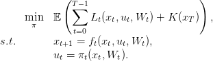
where xt ∈ 𝕏 is the state at time t of the system and ut ∈ 𝕌 the control applied at time t; ft is the dynamics of the system. We assume that the sets 𝕌 and 𝕏 are compact subset of a finite dimensionnal vector space. We also assume that the functions ft are linear. At each time t there is a convex cost Lt(xt,ut) that depends on the current state and the control choosen. Moreover there is a final cost K(xT ) that depends on the final state of the system. A policy is a sequence of functions π = (π1,…,πT−1) giving for any state x a control u.
We consider the following problem
 | (4) |
This problem can be solved by dynamic programming.
Question 3 Write the Dynamic Programming equation relative to this problem. How to compute the Bellman Value function ? How to compute the optimal policy ?
In order to understand the SDDP algorithm it is useful to introduce the Bellman operator 𝒯t of the problem.
For any time t, and any function A mapping the set of states into ℝ we define:
 | (5) |
Question 4 Write the Dynamic Programming equation with the Bellman operator.
Let study a few properties of the Bellman operator.
Monotonicity For any couple of functions (V,V ), we have
 | (6) |
Convexity For any function V , if Lt is jointly convex in (x,u), V is convex, and ft is affine then
 | (7) |
Linearity For any piecewise linear function  , if
, if  is also piecewise linear, and ft affine,
then
is also piecewise linear, and ft affine,
then
 | (8) |
Question 5 Prove these three results.
Let J be a function mapping 𝕏 × 𝕌 into ℝ. Consider the function φ defined as
where J is jointly convex in (x,u). Then the interpretation of the multiplier as a marginal cost implies that a subgradient λ ∈ ∂φ(x0) of φ at x0 is the dual multiplier of constraint x0 − x = 0 in the following problem
 |
In particular it means that, as φ is convex
 | (9) |
As in the Kelley’s algorithm, the SDDP algorithm recursively constructs a lower-approximation
 t(k) of each Bellman function V
t as the supremum of a number of affine functions. Each of this
affine functions is called a cut.
t(k) of each Bellman function V
t as the supremum of a number of affine functions. Each of this
affine functions is called a cut.
Stage k of the SDDP algorithm goes as follows.
Suppose that we have a collection of T lower approximation of the Bellman functions denoted
 t(k) that is a maximum of affine functions. In order to improve our approximation we follow an
optimal trajectory (xt(k))
t of the approximated problem and add a cut computed along the optimal
trajectory for each Bellman function.
t(k) that is a maximum of affine functions. In order to improve our approximation we follow an
optimal trajectory (xt(k))
t of the approximated problem and add a cut computed along the optimal
trajectory for each Bellman function.
Thus, we begin with a loop forward in time by setting t = 0 and xt(k) = x 0, and solve
 |
We call βt(k+1) the value of the problem, λ t(k+1) a multiplier of the constraint x = x t(k), and u t(k) an optimal solution. This can also be written as
 |
Thus we have by (9), and by monotonicity of 𝒯t,
 | (11) |
This ensures that the function x βt(k+1) +
  is indeed a cut, i.e an affine function
below V t. Consequently we update our approximate of V t by defining
is indeed a cut, i.e an affine function
below V t. Consequently we update our approximate of V t by defining

Furthermore we can see that  t(k+1) is convex and lower than V
t. We go to the next time step by
setting
t(k+1) is convex and lower than V
t. We go to the next time step by
setting
In order to initialize the algorithm it seems that we need a lower bound to all value function. According to our assumptions this bound always exist but is not necessary in order to implement the algorithm. Indeed we can choose V t(0) = 0 in order to compute the trajectories, and simply set V t(1) equal to the first cut, which means that we “forget” V (0) in the maximum that determine V t(1).
Note that at any step k of the algorithm we have a (non optimal) solution (u(k)) t of Problem (4), and we can estimate the quality of the solution. Indeed V 0(k)(x 0) is a lower bound to the optimal value of Problem (4). Moreover the simulated cost following the solution given by
Now we introduce some random variables in our problem. This complexify the algorithm in different ways:
As in the deterministic case we consider a controled stochastic dynamic system in discrete time that follows the equation

where xt ∈ 𝕏 is the state at time t of the system, ut the control applied at time t, and Wt an exogeneous discrete noise ; ft is the dynamic of the system.
We assume that the stochastic process (Wt)t=1,…,T−1 is independent in time. Moreover we assume that at any time t we know the whole past of the noise process up to, and including, time t. The independence assumption ensures that we can only consider control ut measurable with respect to (xt,Wt). This is the so called hazard-decision information structure where we know at time t the realization of the noise before choosing our control.
At each time t there is a jointly convex in (xt,ut) cost, Lt(xt,ut,Wt) that depends on the current state and the control choosen ; and there is a final cost K(xT ) the depends on the final state of the system. A policy is a sequence of measurable functions π = (π1,…,πT−1) giving for any state x, and realization of the noise w a control u.
We consider the following problem
 | (12) |
As in the deterministic case we also introduce the stochastic Bellman operator 𝒯t of the problem. For any time t, and any function A mapping the set of states and noises 𝕏 × 𝕎 into ℝ we define:

The stochastic Bellman operator 𝒯t, is given by

Question 7 Write the Dynamic Programming used to solve this problem in two ways: directly, and with the help of the Bellman operator.
Question 8 Show that the Bellman operator have the same properties as in the deterministic case.
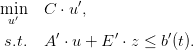
Suppose that for an iteration k and a time step t + 1 we have a lower estimation V t+1k+1 of V t+1. We consider, for any w, the problem
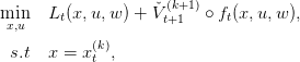 | (13) |
and call  t(k+1)(w) the optimal value, and
  t(k+1)(w) an optimal multiplier of the constraint. As in
the deterministic case we have
t(k+1)(w) an optimal multiplier of the constraint. As in
the deterministic case we have
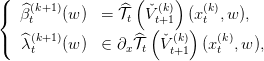 | (14) |
At the beginning of step k we suppose that we have, for each time step t an approximation  t(k) of
V t verifying
t(k) of
V t verifying
 t(k) ≤ V
t,
t(k) ≤ V
t,
 t(k) is convex.
Forward path We randomly select a scenario (w0,…,wT−1) ∈ 𝕎T . We recursively, by a forward loop in time, define a trajectory (xt(k)) t=0,…,T by xt+1(k) = f t(xt(k),u t(k),w t), where ut(k) is an optimal solution of
 | (17) |
This trajectory is a trajectory given by the optimal policy of Problem (12) where V t is replaced by
its current approximation  t(k).
t(k).
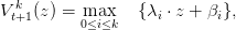
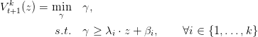
Backward path
We reader improve the approximation of V t by adding a cut at V t(xt(k)). We procede backward
in time by setting t = T − 1, and solve Problem (13) for every w in the support of Wt. We obtain
 t(k+1)(w) and
  t(k+1)(w). As W
t is discrete we can compute exactely the expectation λt(k+1) and
βt(k+1), and define the new lower approximation
t(k+1)(w). As W
t is discrete we can compute exactely the expectation λt(k+1) and
βt(k+1), and define the new lower approximation

Question 10 Check that  t(k+1) is a lower convex approximation of V
t.
t(k+1) is a lower convex approximation of V
t.
Question 11 For one iteration of the SDDP, algorithm, how many one-step one-alea problem (Problem (17)) do we need to solve ?
We can intialize as suggested in the deterministic case. However in order to accelerate the convergence it can be useful to bypass a few forward paths by abritrarily choosing some trajectories (xt(k)) t.
As in the deterministic case we have an exact lower bound of Problem (12) given by V 0(k)(x 0). However, determining an upper bound is more difficult. Indeed, the upper bound is given as the expectation of the cost induced by the optimal strategy of the approximated problem. This expectation is to be taken on the whole process (W0,…,WT−1) and cannot be computed exactly. Consequently this expectation is estimated by Monte-Carlo methods, and we have no control over the error of our solution.
A heuristic stopping rule consist in stopping the algorithm if the lower bound is in the confidence interval of the upper bound for a determined number of Monte-Carlo simulation.
In the algorithm presented here, also called DOASA, we select one scenario (one realization of (W1,…,WT−1)) to do a forward and backward path. It is also possible to select a number N of scenarios to do the forward path (computation can be parallelized). Then during the backward path we add N cuts to V t before computing the cuts on V t−1. This is the original implementation of the algorithm.
Otherwise the CUPPS algorithm suggest to use  t+1(k) instead of V
t+1(k+1) in the
computation of the cuts (14). In practice it means that we do only a forward path at step k:
t+1(k) instead of V
t+1(k+1) in the
computation of the cuts (14). In practice it means that we do only a forward path at step k:
Moreover it is possible to select more than one scenario, and everything can be parralelized in this implementation.
Finally it is always possible, and most of the time fruitful to compute some cuts before starting the algorithm. One way of doing this is to bypass the forward phase by choosing the trajectory (xt(k)) t=0,…,T instead of computing it as some optimal trajectory.
We consider a dam manager intenting to minimize the intertemporal cost obtained by turbining the water in a dam, when the water inflow (rain, outflows from upper dams) is supposed to be stochastic.
 |
with
![𝕏 = [0,S ♯]](sddp53x.png) , made of water volumes (h m3), where
, made of water volumes (h m3), where  is the maximum dam volume,

 , and supposed to be known at the beginning of the period
(Hazard-Decision),
, and supposed to be known at the beginning of the period
(Hazard-Decision),
![𝕌 = [0,q♯]](sddp57x.png) , where q♯ is the maximum which can be turbined by
time unit (and produce electricity),
, where q♯ is the maximum which can be turbined by
time unit (and produce electricity),
 , and such that
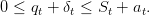 | (18) |
The dam manager is supposed to make a decision, here turbining qt and spilling δt, at the beginning of the period [t,t + 1], after knowing the water inflow at.
A water inflows scenario is a sequence as
 | (19) |
Compared to other methods, we have added the spilled outflow volume δ in order to get a linear dynamics and we are placed in the Hazard-Decision case. These two points are mandatory to apply the SDDP algorithm.
The manager original problem is one of cost minimization where turbining one unit of water has unitary cost −pt. On the period from t0 to T, the costs sum up to
 | (20) |
where
 | (21) |
is given (data of the problem) and supposed to be known in advance (deterministic setting),
 gives value to the water volume in the dam at the horizon T.
We suppose that sequences of uncertainties (at0,…,aT−1) are random variables with a known probability distribution ℙ on the set {0,…,a♯}, with ℙ{a t = a} given.
Notice that the random variables (at0,…,aT−1) are independent, but that they are not necessarily identically distributed. This allows us to account for seasonal effects (more rain in autumn and winter).
We now perform numerical simulations, and try different policies.
Time. We consider a daily management over one year
 | (22) |
Bounds. Concerning the dam and water inflows, we consider the following bounds:
 | (23) |
These figures reflect the assumptions that, during one week, one can release at maximum 40% of the dam volume, and that during one week of full water inflows, an empty dam can be half-filled.
Costs scenario.
The scenario  of costs is known in advance. We produce it by one
sample from the expression
of costs is known in advance. We produce it by one
sample from the expression
 | (24) |
where  is drawn from a sequence of i.i.d. uniform random variables in
 ![[− 1∕2, 1∕2]](sddp69x.png) .
.
Water inflow scenarios.
We produce scenarios a(⋅) :=  at0,…,aT−1
 of water inflows by a sequence of independent
random draws from the set {0, 1,
of water inflows by a sequence of independent
random draws from the set {0, 1, ,a♯}.
,a♯}.
An admissible policy π : 𝕋 × 𝕏 × 𝕎 → 𝕌 × 𝔻 assigns an amount of water turbined and spilled
 to any state S of dam stock volume, to any decision period t ∈ 𝕋 and to any
water inflow a ∈ 𝕎, while respecting the constraints
to any state S of dam stock volume, to any decision period t ∈ 𝕋 and to any
water inflow a ∈ 𝕎, while respecting the constraints
 | (25) |
that can also be written
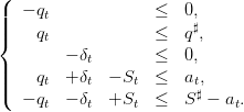 | (26) |
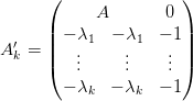
The system (26) is equivalent to
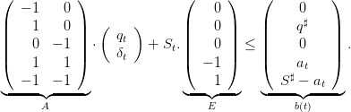 | (27) |
In the following, we will simply write as defined A ⋅ + St.E ≤ b(t).
Once the policy given, we obtain a volume trajectory S(⋅) =  , a turbined
trajectory q(⋅) =
, a turbined
trajectory q(⋅) =  and a spilled trajectory δ(⋅) =
  produced by
the ”closed-loop” dynamics
produced by
the ”closed-loop” dynamics
 | (28) |
and function of the scenario a(⋅). Thus, in the end, we obtain the cost
 | (29) |
The aim of this part is to compute the minimum of a given convex function under linear constraints and to find a cutting plane. We will use this to find an optimal strategy.
The problem is
 | (30) |
In order to use the linear solver, we have to transform this formula into one of the form
 | (31) |
We remind the reader that V t+1k is a piecewise linear function written
 | (32) |
By writting
 ,
,  ,
,  and
and 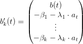 ,
we obtain the wanted form for the minimization problem (see (31)).
,
we obtain the wanted form for the minimization problem (see (31)).
The last step is to find the parameters of the cutting plane of the Bellman function V tk at a given point z. To do so, we transform the state z in the previous equation in a variable x and add the constraint x = z. The Lagrange multiplier of this equality constraint is the slope of a new cutting plane and the minimum cost is the ordinate at the origin.
The following macro returns the parameters of the plane (λ,β) and the point at which the minimum is reached uopt given the matricial form of the cost (−p,V ), the constraints (A,b(t),E), the value of the uncertainty a, the dynamics given by (Q,R) and the state z.
Question 12 Explain the objective of the function CutPerAlea. Where, in the SDDP algorithm, is this function required ? How many times is the function called for a step k of the SDDP algorithm ?
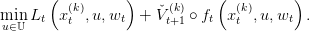
We now solve the problem presented earlier in this practical work, by Dynamic Programming and by Stochastic Dual Dynamic Programming.
Question 13 First of all open the file damdata.sce, and understand the different macro given in this file, in particular the macro trajectories.
Now define a policy (a function taking a time t, a current stock s and an inflow a and giving an admissible control), and test it. Plot (using plot2d2) the trajectories of the stock with this policy.
We solve exactly the problem using Dynamic Programming.
Question 14 In the file sdp.sce a Dynamic Programming approach is presented. Understand how the function works, and plot the optimal stock trajectory using function from damdata.sce.
From the function of sdp.sce what is the exact value of the optimization problem ? Simulate the optimal strategy and give an estimation of this value and asymptotic error bounds.
What do you observe for the final stock? Explain why.
We now apply an SDDP approach to the same problem.
In the files that were downloaded at the beginning, the function SDDP creates an approximate of the Bellman function given the constraints and random trajectories, then the function sddp_policy defines the optimal policy given the former approximate.
Question 15 Using the function of SDDP picture the trajectory of the stocks corresponding to the optimal policy. Evaluate the optimal payoff, and the error bounds.
Evaluate the lower bound given by SDDP. Deduce the estimated gap (in %).
Plot the improvement of the gap with iterations of SDDP.
Question 16 Compare the numerical results given by the DP approach, and the SDDP approach.
Sum up the theoretical and practical differences between DP and SDDP: what are the pros and cons of each method.