1 Problem statement
We formalize the problem of fixing energy reserves in a day-ahead market as a two stage stochastic
optimization problem. A decision has to be made at night of day J — which quantity of the
cheapest energy production units (reserve) to be mobilized — to meet a demand that will
materialize at morning of day J + 1. Excess reserves are penalized; demand unsatisfied by reserves
have to be covered by costly extra units. Hence, there is a trade-off to be assessed by
optimization.
1.1 Stages
There are two stages, represented by the letter t (for time):
- t = 0 corresponds to night of day J;
- t = 1 corresponds to morning of day J + 1.
1.2 Probabilistic model
We suppose that the demand, materialized on the morning of day J + 1, can take a
finite number S of possible values Ds, where s denotes a scenario in the finite set 𝕊
(S=card(𝕊)).
We denote πs the probability of scenario s, with
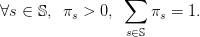 | (1) |
Notice that we do not consider scenarios with zero probability.
1.3 Decision variables
The decision variables are the scalar Q0 and the finite sequence  s∈𝕊 of scalars, as follows:
- at stage t = 0, the energy reserve is Q0;
- at stage t = 1, a scenario s materializes and the demand Ds is observed, so that one
decides of the recourse quantity Q1,s.
The decision variables can be considered as indexed by a tree with one root (corresponding to the
index 0) and as many leafs as scenarios in 𝕊 (each leaf corresponding to the index 1,s): Q0
is attached to the root of the tree, and each Q1,s is attached to a leaf corresponding
to s.
1.4 Optimization problem formulation
The balance equation between supply and demand is
 | (2) |
The energies mobilized at stages t = 0 and t = 1 display different features:
- at stage t = 0, the energy production has maximal capacity Q0♯, and producing Q
0
costs 𝒞0(Q0);
- at stage t = 1, the energy production is supposed to be unbounded, and producing Q1
costs 𝒞1(Q1).
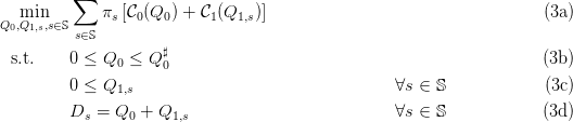
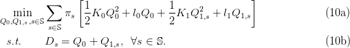
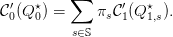
We consider the stochastic optimization problem
Here, we look for energy reserve Q0 and recourse energy Q1,s so that the balance
equation (3d) is satisfied (at stage t = 1) at minimum expected cost in (3a). By weighing each
scenario s with its probability πs, the optimal solution  performs a compromise
between scenarios.
performs a compromise
between scenarios.
2 Formulation on a tree with linear costs
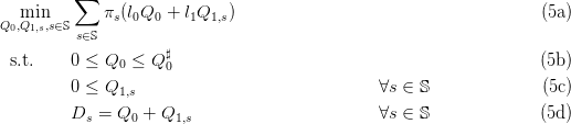
Here, we suppose that the costs are linear:
 | (4) |
Therefore, the stochastic optimization problem (3) now becomes
This optimization problem (5) is linear. When the number S of scenarios is not too large, we
can use linear solvers.
Question 1 We consider the case when 𝕊 = {L,M,H} has S = 3 scenarios (low, medium, high).
We want to transform the linear optimization problem (5) under a form adapted to a linear
solver.
-
a)
- [1+1+1] Expand the criterion (5a). Expand the inequalities (5b)–(5c) into an
array of five scalar equations (one inequality per equation), and the equalities (5d) into
an array of three scalar equations (one equality per equation).
-
b)
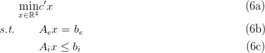
- [1+1+1+1+1] Let x be the column vector x = (Q0,Q1L,Q1M,Q1H). Propose
matrices Ae, Ai and column vectors be, bi and c such that the linear optimization problem (5)
can be written under the form
Question 2 We are going to numerically solve the linear optimization problem (5).
-
a)
- [2] Interpret the code below. What is the macro linpro doing? What is lopt? Copy
the code into a file named tp_q1.sce.
-
b)
- [1+2] Solve a numerical version of problem (5) with S = 3 scenarios and the
parameters in the code below, by executing the file tp_q1.sce. What is the optimal
value Q0⋆ of the reserve? What is the optimal value Q
1,L⋆? Can you explain why these
values are optimal? (there is an economic explanation based on relative costs; there is a
mathematical explanation based on the properties of the solutions of a linear program).
-
c)
- [3] Then, increase and decrease the value of the unitary cost l1 (especially above
and below l0). Show the numerical results that you obtain. What happens to the optimal
values Q0⋆? Explain why (make the connection with the properties of the solutions of a
linear program).
S=3; q0m=30;
if S==3 then D=[15;20;50]; Pr=[0.2;0.6;0.2];
else D=grand(S,1,'uin',5,50); Pr=grand(S,1,'unf',0,1);
Pr=Pr ./sum(Pr); end
ll0=2;ll1=5;
c=[ll0;ll1 .*Pr];
Ai=[-eye(S+1,S+1);eye(1,S+1)]; bi=[zeros(S+1,1);q0m];
Ae=[ones(S,1),eye(S,S)];
be=[D];
A=[Ae;Ai];b=[be;bi];
[xopt,lopt,fopt]=linpro(c,A,b,[],[],size(be,'*'))
Question 3 We are going study the impact of the number S of scenarios on the numerical
resolution of the linear optimization problem (5).
-
a)
- [2] Take S = 100. What is the optimal value Q0⋆ of the reserve? Identify the
scenario s with the lowest demand. What is the optimal value Q1,s⋆? Explain.
-
b)
- [1] For what value of n in S = 10n can you no longer solve numerically?
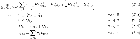
3 Formulation on a tree with quadratic convex costs
Here, we suppose that the costs are quadratic and convex:
 | (7) |
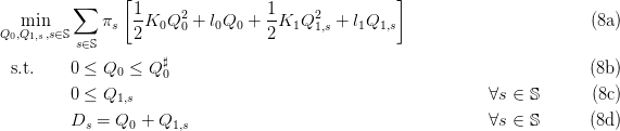
The optimization problem (3) is quadratic convex:
When the number S of scenarios is not too large, we can use quadratic solvers.
Question 4 We are going to numerically solve the quadratic convex optimization problem (8).
-
a)
- [1] Interpret the code below. What is the macro quapro doing? Copy the code into
a file named tp_q2.sce.
-
b)
- [1] Solve a numerical version with S = 3 scenarios and the parameters in the code
below, by executing the files tp_q1.sce and tp_q2.sce. What is the optimal value Q0⋆ of
the reserve? What is the optimal value Q1,L⋆?
-
c)
- [1+1+2] Check numerically that
 is an inner solution to
the optimization problem (8a), that is, check numerically that the inequalities (8b) and
(8c) are strict. What is the difference with the optimal solution of Question 2? Discuss the
difference (make the connection with the properties of the solutions of a linear program).
is an inner solution to
the optimization problem (8a), that is, check numerically that the inequalities (8b) and
(8c) are strict. What is the difference with the optimal solution of Question 2? Discuss the
difference (make the connection with the properties of the solutions of a linear program).
-
d)
- [2+1] Compute the derivatives of the cost functions in (7). Check numerically (giving the
details of computation) that the optimal solution
 satisfies the following
relation between marginal costs:
satisfies the following
relation between marginal costs:
 | (9) |
exec('tp_q1.sce');
A=[Ae;Ai];b=[be;bi]; KK0=10;KK1=1; KK=diag([KK0,KK1*Pr' .*ones(1,S)]);
[xopt,lopt,fopt]=quapro(KK,c,A,b,[],[],size(be,'*'))
Question 5 We are going to numerically solve the quadratic convex optimization problem (8)
after changing the relative values of the (quadratic) parameters K0 and K1. For the
parameters K0, l0, l1, we take the same values as those in Question 2 (hence l1 > l0) and in
Question 4.
-
a)
- [1] Take K1 > K0 with K1 ≈ K0. What are the optimal value Q0⋆ of the reserve
and the optimal value Q1,L⋆?
-
b)
- [1] Take K1 > K0 with K1 >> K0. What are the optimal value Q0⋆ of the reserve
and the optimal value Q1,L⋆?
-
c)
- [2] Discuss.
Question 6 We are going study the impact of the number S of scenarios on the numerical
resolution of the quadratic convex optimization problem (8).
-
a)
- [1] Take S = 100. Solve a numerical version of problem (8) with the parameters K0,
l0, K1, l1 as in the code of Question 4. What is the optimal value Q0⋆ of the reserve?
Identify the scenario s with the lowest demand. What is the optimal value Q1,s⋆?
-
b)
- [1] For what value of n in S = 10n can you no longer solve numerically?
Question 7 This theoretical question may be ignored
(by those who want to focus on numerical results)
For this question, we temporarily ignore the inequalities (8b) and (8c) in (8). Therefore, we
consider the optimization problem (8a) with equality constraints (8d), that is:
-
a)
- [2] Compute the Hessian matrix of the criterion
![[ ]
S ∑ 1- 2 1- 2
J0 : (Q0, (Q1,s)s∈𝕊) ∈ ℝ × ℝ ↦→ πs 2K0Q 0 + l0Q0 + 2 K1Q 1,s + l1Q1,s .
s∈𝕊](stochastic_programming_energy14x.png) | (11) |
What are the dimensions of the Hessian matrix?
-
b)
- [3] Why does optimization problem (10) have a solution? (Beware of the domain)
-
c)
- [2] Why is the solution unique?
-
d)
- [1+2] Why are the equality constraints (10b) qualified? Why does an optimal solution
 of (10) satisfy the Karush-Kuhn-Tucker (KKT) conditions (first-order
optimality conditions)?
of (10) satisfy the Karush-Kuhn-Tucker (KKT) conditions (first-order
optimality conditions)?
-
e)
- [2] Why is a solution of the KKT conditions an optimal solution of (10)?
-
f)
- [1] Write the Lagrangian
 associated with problem (10).
-
g)
- [2] Deduce the KKT conditions. Show that there exist (μs⋆,s ∈ 𝕊) such that
 | (12) |
-
h)
- [2] Deduce that — when
 is an inner optimal solution to problem (8a) —
we have the following relation between marginal costs:
is an inner optimal solution to problem (8a) —
we have the following relation between marginal costs:
 | (13) |
Give an economic interpretation of this equality.
4 Formulation on a fan with quadratic convex costs
When the number S of scenarios is too large, Problem (5) — be it linear or convex — cannot be
solved by direct methods.
4.1 Dualization of non-anticipativity constraints
To bypass this problem, we use a “trick” consisting in introducing new decision variables  s∈𝕊,
instead of the single decision variable Q0, and we write
s∈𝕊,
instead of the single decision variable Q0, and we write
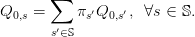 | (14) |
These equalities are called the non-anticipativity constraints. Indeed, the equations (14) express
that
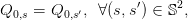 | (15) |
that is, the decision at stage t = 0 does not depend on the scenario s, hence cannot anticipate the
future. Later, we will treat the constraints (14) by duality.
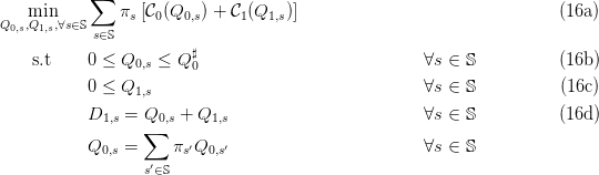
Therefore, the stochastic optimization problem (3) now becomes
By the assumption (1) that there are no scenarios with zero probability (πs > 0), we replace
each equality in the last equation by the equivalent one
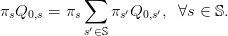 | (16e) |
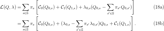
We attach, to each equality above a multiplier λ0,s. We put
 | (17) |
The corresponding Lagrangian is
Question 8 This theoretical question may be ignored
(by those who want to focus on numerical results)
When the costs are quadratic and convex as in (7), show that
-
a)
- [3] the criterion
![[ ]
S S ∑ 1 2 1 2
J : Q ∈ ℝ × ℝ ↦→ πs 2K0Q 0,s + l0Q0,s + 2-K1Q 1,s + l1Q1,s
s∈𝕊](stochastic_programming_energy27x.png) | (19) |
in (16a) is a-strongly convex in  , and provide a possible a > 0,
-
b)
- [2] the domain defined by the constraints in the optimization problem (16) is
closed,
-
c)
- [2] the domain defined by the constraints in the optimization problem (16) is
convex,
-
d)
- [2+1] the optimization problem (16) has a solution, and it is unique, denoted
by Q⋆,
-
e)
- [1] there exists a multiplier λ⋆ such that (Q⋆,λ⋆) is a saddle point of the Lagrangian ℒ
in (18).
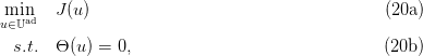
4.2 Uzawa algorithm
We consider the following optimization problem
under the assumptions that
- the set 𝕌ad is a closed convex subset of a Euclidian space ℝN,
- the criterion J : ℝN → ℝ is an a-strongly convex (a > 0) and differentiable function,
- the constraint mapping 𝜃 : ℝN → ℝM is affine, κ-Lipschitz (κ > 0),
- the Lagrangian ℒ(u,λ) = J(u) + ⟨λ, Θ(u)⟩ admits a saddle-point over 𝕌ad × ℝM.
Then the following algorithm — called dual gradient algorithm, or Uzawa algorithm — converges
toward the optimal solution of Problem (20), when 0 < ρ < 2a∕κ2.
Data: Initial
multiplier
λ(0),
step
ρ
Result: optimal
decision
and
multiplier;
repeat
u(k) = arg min
u∈𝕌adℒ(u,λ(k))
;
λ(k+1) = λ(k) + ρΘ(u(k))
;
until Θ(u(k)) = 0;
Algorithm .1: Dual Gradient Algorithm
4.3 Numerical resolution by Uzawa algorithm (quadratic convex case)
When the costs are quadratic and convex as in (7), the optimization problem (16) becomes:
Question 9 This theoretical question may be ignored
(by those who want to focus on numerical results)
When the costs are quadratic and convex as in (7), identify in the optimization problem (21) the
corresponding elements in the Uzawa algorithm .1:
-
a)
- [1] decision variable u,
-
b)
- [1] decision set ℝN (for what N?),
-
c)
- [2] affine constraints mapping Θ : ℝN → ℝM, corresponding to the constraints (21e)
(why is it κ-Lipschitz, and for which κ?).
-
d)
- [3] Explain why the Uzawa algorithm converges towards the optimal solution of
Problem (21).
S=3; q0m=30; if S==3 then
D=[15;20;50]; Pr=[0.2;0.6;0.2]; else D=grand(S,1,'uin',5,50);
Pr=grand(S,1,'unf',0,1); Pr=Pr ./sum(Pr); end
ll0=2;ll1=5; KK0=10;KK1=1;
Q0=zeros(S,1); Q1=zeros(S,1); f0=zeros(S,1);
rho=5; lambda=zeros(S,1); for it=0:30 do
for ss=1:S do
ll=[ll0*Pr(ss);ll1*Pr(ss)]; Ai=[-eye(2,2);eye(1,2)];
bi=[zeros(2,1);q0m];
Ae=[1,1]; be=[D(ss)]; A=[Ae;Ai];b=[be;bi]; KK=Pr(ss)*diag([KK0,KK1]);
cc=ll+Pr(ss)*[lambda(ss)-sum(Pr .*lambda);0];
[xopt,lopt,fopt]=quapro(KK,cc,A,b,[],[],size(be,'*')); Q0(ss)=xopt(1);
Q1(ss)=xopt(2); f0(ss)=fopt; printf("Dual function %f\n",sum(f0));
end Q0bar=sum(Pr .*Q0); lambda=lambda+rho*(Pr .*(Q0-Q0bar)); end
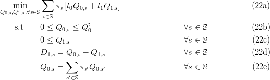
5 Formulation on a fan with linear costs
Here, we suppose that the costs are linear, as in (4).
5.1 Difficulties in applying Uzawa algorithm with linear costs
The optimization problem (16) becomes:
Question 11 We are going to numerically solve the linear optimization problem (22).
-
a)
- [2] Detail what the code below is doing. Why do we use the macro linpro? Copy the
code into a file named tp_q4.sce.
-
b)
- [3] Solve a numerical version with S = 3 scenarios. What do you observe regarding
convergence of the Uzawa algorithm? Can you explain why?
S=3; q0m=30; D=[15;20;50];
Pr=[0.2;0.6;0.2]; rho=0.1;
ll0=2;ll1=5;
Q0=zeros(S,1); Q1=zeros(S,1); f0=zeros(S,1);
lambda=zeros(S,1); for it=0:30 do for ss=1:S do
ll=[ll0*Pr(ss);ll1*Pr(ss)]; Ai=[-eye(2,2);eye(1,2)];
bi=[zeros(2,1);q0m]; Ae=[1,1];
be=[D(ss)]; A=[Ae;Ai];b=[be;bi]; cc=ll+Pr(ss)*[lambda(ss)-sum(Pr .*lambda);0];
[xopt,lopt,fopt]=linpro(cc,A,b,[],[],size(be,'*')); Q0(ss)=xopt(1);
Q1(ss)=xopt(2); f0(ss)=fopt; printf("Dual function %f\n",sum(f0));
end Q0bar=sum(Pr .*Q0); lambda=lambda+rho*(Pr .*(Q0-Q0bar)); end
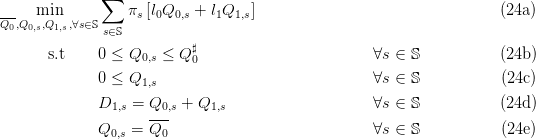
5.2 Dualization of non-anticipativity constraints
To bypass the difficulty in applying Uzawa algorithm with linear costs, we use a “trick” consisting
in introducing new decision variables Q0 and  s∈𝕊, instead of the single decision variable Q0,
and we write
s∈𝕊, instead of the single decision variable Q0,
and we write
 | (23) |
These equalities are another form of the non-anticipativity constraints. Indeed, the equations (23)
express that the decision at stage t = 0 cannot anticipate the future, hence cannot depend on the
scenario s. We will treat these constraints by duality.
Therefore, the stochastic optimization problem (3) now becomes
By the assumption (1) that there are no scenarios with zero probability (πs > 0), we replace
each equality in (24e) by the equivalent one
 | (25) |
We attach, to each equality above a multiplier λ0,s. We put
 | (26) |
5.3 Augmented Lagrangian and obstacles to decomposition
5.4 Progressive Hedging algorithm (quadratic solver)
Question 12 We are going to numerically solve the linear optimization problem (24) by the
Progressive Hedging algorithm.
-
a)
- [3] Detail what the code below is doing. Why do we use the macro quapro? Explain
the two roles of the new parameter rr. Copy the code into a file named tp_q5.sce.
-
b)
- [2] Solve a numerical version with S = 3 scenarios. What do you observe regarding
convergence of the Uzawa algorithm? Can you explain why?
S=3; q0m=30; D=[15;20;50];
Pr=[0.2;0.6;0.2];
ll0=2;ll1=5;
rr=0.1;
Q0=zeros(S,1); Q1=zeros(S,1); f0=zeros(S,1);
lambda=zeros(S,1); Q0bar=0; for it=0:300 do
for ss=1:S do
ll=[ll0*Pr(ss);ll1*Pr(ss)];
Ai=[-eye(2,2);eye(1,2)]; bi=[zeros(2,1);q0m];
Ae=[1,1]; be=[D(ss)];
A=[Ae;Ai];b=[be;bi]; KK=rr*Pr(ss)*diag([1,0]); cc=ll+[Pr(ss)*lambda(ss);0];
cc=cc+[-rr*Q0bar*Pr(ss)]; [xopt,lopt,fopt]=quapro(KK,cc,A,b,[],[],size(be,'*'));
Q0(ss)=xopt(1); Q1(ss)=xopt(2); f0(ss)=fopt; end
Q0bar=sum(Pr .*Q0); lambda=lambda+rr*(Pr .*(Q0-Q0bar));
end Q1=max(0,(D-Q0bar));
5.5 Progressive Hedging algorithm (linear solver)
A Additional code for “Formulation on a tree with linear costs”
S=3; q0m=30;
if S==3 then D=[15;20;50]; Pr=[0.2;0.6;0.2];
else D=grand(S,1,'uin',5,50); Pr=grand(S,1,'unf',0,1);
Pr=Pr ./sum(Pr); end
ll0=2;ll1=5;
c=[ll0;ll1 .*Pr];
Ai=[-eye(S+1,S+1);eye(1,S+1)]; bi=[zeros(S+1,1);q0m];
Ae=[ones(S,1),eye(S,S)];
be=[D];
if exists('%nsp') then [xopt,fopt,flag]=linprog(c,Ai,bi,Ae,be);
if exists('quapro','callable') then A=[Ae;Ai];b=[be;bi];
[xopt_q,lagr_q,fopt_q]=quapro(zeros(S+1,S+1),c,A,b,[],[],size(be,'*'))
end else A=[Ae;Ai];b=[be;bi];
[xopt,lopt,fopt]=linpro(c,A,b,[],[],size(be,'*')) end
B Additional code for “Formulation on a tree with quadratic convex costs”
if exists('%nsp') then load_toolbox('quapro'); end
exec('tp_q1.sce');
A=[Ae;Ai];b=[be;bi]; KK0=10;KK1=1; KK=diag([KK0,KK1*Pr' .*ones(1,S)]);
if exists('%nsp') then
if exists('quapro','callable') then [xopt_q,lagr_q,fopt_q]=quapro(KK,c,A,b,[],[],size(be,'*'))
end else [xopt,lopt,fopt]=quapro(KK,c,A,b,[],[],size(be,'*'))
end
function [f,g,ind]=costf(q0,ind) q1=max(0,(D-q0));
f=sum(Pr .*(ll0*q0+ll1*q1))+(1/2)*[q0;q1]'*KK*[q0;q1]
g=sum(Pr .*(ll0-ll1*(D-q0 >= 0)))+KK(1,1)*q0+-sum((D-q0 >= 0) .*(KK(2:$,2:$)*q1))
endfunction if exists('%nsp') then Q0=optim(costf,0,xinf = 0,xsup = q0m) else
[fo,Q0]=optim(costf,'b',0,q0m,0) end Q1=max(0,(D-Q0))
 given by the algorithm? Do you have that
  , for all
 ?
?