A decomposition-coordination method
for the cascade interconnected dams problem

Sowg
(last modiﬁcation date: October 10, 2017)

Version pdf de ce document
Version sans bandeaux

Hydroelectricity is the main renewable energy which is produced in France (over 10% of the country annual production). It provides a clean (no greenhouse gases emissions) and fast-usable energy that is cheap and substitutable for the thermal one. We address the question of the production management of cascade-interconnected dams by means of a ﬁnite-horizon Markov decision process. Solving such a problem is not straightforward since it displays a large size, so is likely to suﬀer from the curse of dimensionality. We handle it with a decomposition-coordination algorithm that we adapt by approximation to the stochastic case.

1 Description of the problem
2 Exact solution by dynamic programming
3 Approximate solution by dual approximate dynamic programming

1 Description of the problem
1.1 Dynamics of a single dam and dams cascade
1.2 The optimization problem
1.3 Numerical instance
2 Exact solution by dynamic programming
3 Approximate solution by dual approximate dynamic programming
3.1 Dualization of the coupling constraint and DADP
3.2 A heuristic to construct an admissible solution

Introduction

This pratical work will follow the lecture entitled Decomposition-coordination methods in stochastic optimal control (P. Carpentier). The computations will be performed using nsp and only nsp. In order to launch nsp write nsp & in a terminal. Type pwd to see the current repertory and then download the practical work material from the Internet to this repertory. Since we will use a three dimension dynamic programming algorithm, a part of the programming functions had to be written in C. Moreover, we have to load some scenarios datas. Thus, we will need a speciﬁc nsp toolbox called COURSES/stochdec. In order to load it, go to the stochdec repertory and type exec('loader.sce');.

1 Description of the problem

1.1 Dynamics of a single dam and dams cascade

Let time t vary in {0,...,T}. The following real valued random variables are deﬁned on a probability space (Ω, ℱ,ℙ ) :

X_tⁱ is the storage level at the beginning of period [t,t + 1); (state)
U_tⁱ is the hydroturbine outﬂow during [t,t + 1); (production control)
Z_tⁱ is the inﬂow from dam i − 1 into dam i during [t,t + 1); (coordination control)
W_tⁱ is the exogeneous inﬂow into dam i during [t,t + 1).; (noise)

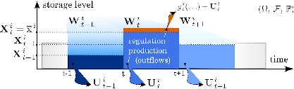
The dynamics of the dam reads:

Xi = min {Xi + Wi + Zi − Ui ,xi} with Xi := xi. t+1 t t t t 0 0

(1)

When X_tⁱ + W_tⁱ + Z_tⁱ −U_tⁱ is greater than xⁱ, the diﬀerence is spilled from dam i to dam i + 1 so that the upper bound constraint on dam i is directly handled by the dynamics. Therefore the total outﬂow from dam i to dam i + 1 is given by:

i( i i i i) { i i i -i i} gt X t,U t,W t,Z t := max X t + W t + Zt − x ,U t .

The bounds constraints are:

-- xi ≤ Xit+1 and 0 ≤ Uit ≤ min {uit,Xit + Wit + Zit − xi}, ∀t ∈ {0, ...,T − 1}.

(2)

Figure 1: Dynamics of dam i

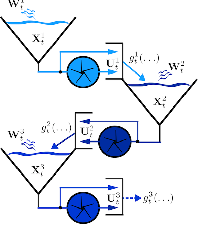
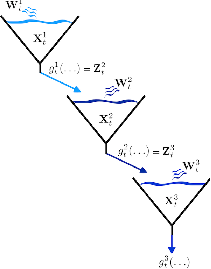
Each dam i ∈{2,…,N} receives from the dam i − 1 outﬂ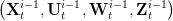ows g_tⁱ⁻¹ ( )
Xit−1,Ui−t 1,Wit−1,Zi−t1 as inﬂows Z_tⁱ and sends its own outﬂows into the dam i + 1 reservoir, at every t ∈{0,…,T}. With the notation Z_t¹ ≡ 0, this leads to the following coupling constraints:

( ) Zit = git−1 Xit−1,Uit−1,Wi −t1,Zi−t 1 ∀ (i,t) ∈ {2, ...,N } × {0, ...,T − 1}.

(3)

Figure 2: Dynamics of three cascade-interconnected dams

1.2 The optimization problem

We assume that the noise random variable W_t = (W_t¹,W_t²,W_t³) are independent over time. The hydroelectric production obeys the following valorization mechanism for every dam:

the production at time t, U_tⁱ, is p_t linearly retributed and a quadratic cost to produce 𝜀 × U_tⁱ² has to be considered,
$Li(Xi ,Ui,Wi ) := − pt × Ui + 𝜀 × Ui2; t t t t t t$
a ﬁnal storage level appreciation function Kⁱ(X_Tⁱ) prevents the reservoir from being lower than a target storage level ⁱ at the end of the study period,
$i i i i i 2 K (X T) := a × max {^x − X T,0} .$

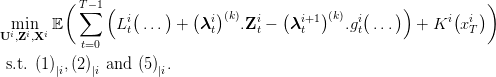
We consider the expected value of the sum of every dam total gain as the problem criterion:

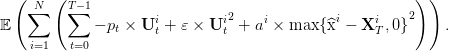( ∑N (T∑− 1 )) 𝔼 − pt × Ui + 𝜀 × Ui 2 + ai × max {^xi − Xi ,0}2 . t=0 t t T i=1

(4)

Note that this criterion is both time and space separable. The control U = (U₀ⁱ,…,U_T−1ⁱ)_i must satisfy the non anticipativity constraint in the hazard-decision framework. So, U_tⁱ has to be measurable with respect to the noises up to time t:

Uit ≼ ℱt where ℱt := (X0, W0, ...,Wt )∀t ∈ {0, ...,T − 1 }.

(5)

The problem consists in minimizing the criterion (4) under the dynamics (1), the coupling (3), the bounds (2) and the measurability (5) constraints.

1.3 Numerical instance

We will test algorithms on a valley composed of three cascade-interconnected dams over a T = 12 time steps period. The problem is of a discrete type and the dams share the following common characteristics:

the volume X_tⁱ of every dam i at t belongs to the forty one integers set ;
the space in which every control U_tⁱ takes its values is discretized over the six integers set ;
the noise random variables W_tⁱ are considered as being interstage independent and uniformely distributed over a ﬁnite set of ten integers.

The simulation part is based on 500 intakes scenarios.

Question 1 Execute the script answer-question1.sce which is stored in the directory COURSES/stochdec. This script will draw N simulation scenarios for the dam number 1. Take a look at the script and change it to draw the scenarios of the other dams.

The contents of the script answer-question1.sce is reproduced here:

  // You should be in COURSES/stochdec to run this script
  exec('loader.sce');
  SIMSCEN=dp_get_simulation_scenarios();

  // get the inflows law on dam 1
  M=fscanfMat('Datas/Generated_datas/generated_intakes_0.txt');

  // QUESTION 1:
  xclear();
  [nss,v]=size(SIMSCEN)
  N=10
  // Draw N scenarions of intakes of dam 1
  Sim=SIMSCEN(1:N,:)+1;// take care to add one
  T=dp_horizon();
  res=Sim;

  for t=1:T-1 do
    res(:,t)=M(Sim(:,t),t);
  end;

  xset('colormap',jetcolormap(N));
  plot2d([],res');
  xtitle(sprintf('first %d simulation scenarios',N));

2 Exact solution by dynamic programming

The noises W_tⁱ are independent over time, so that the problem can be theoretically solved by stochastic dynamic programming (DP). Although, DP is prone to face the curse of dimensionality (the method is not numerically tractable as soon as the number of dams is larger than 5 ) you will ﬁrst solve the three cascade interconnected dams problem by DP since it is numerically possible (as N = 3). Note that the discretization of the problem avoids us to use an interpolation scheme to implement the method.

Question 2 Running DP on the cascade of three connected dams is obtained using the function dp_run(). Then call the function dp_simu() as follows [cost, stocks, controls]=dp_simu() to obtain the expected cost and the stocks and the controls trajectories. Plot the stocks trajectories and show the optimal expected cost. Note that, for example, you will obtain the stocks evolution of dam 1 by using S1=stocks{1}.

Question 3 For the most sceptical of you, just try to beat the DP-computed strategy by building your own strategy ! ;) For example, you may want to multiply the optimal control mapping by a scalar γ ∈ [0,1] to get a new control U (you can use dp_getu(U) and dp_setu(U) to obtain or set the current used control table). Simulate the strategies obtained with your control strategy by using dadp_simu() and compare to what you had obtained before.

Question 4 You can also design your own strategy using function dp_f2u and simulate your strategy as seen in question3. How far is your solution expected cost from the optimal one?

The next script gives some hints on how to use dp_f2u:

  function u=myfeedback(t,w,x)
  // scalar t, vector w of size 4 (three inflows and a price)
  //, vector x of size 3 (water levels of the dams)
     u=sin(t)*x(1)*w(4)*[0;1;0]+x(3);
  endfunction
  // dp_f2u(fn): use a feedback function given as
  // argument to fill a control array U.

  U=dp_f2u(myfeedback)
  ...

3 Approximate solution by dual approximate dynamic programming

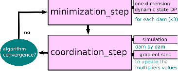
In a few words, we decompose the three dimension dynamic state problem into three one dimension dynamic state problems. This is done by:

dualizing the coupling constraints;
coordinating the local optimal solutions to got the global optimal one using an Uzawa algorithm.

3.1 Dualization of the coupling constraint and DADP

We aim at dualizing (3) and at solving the problem by using an Uzawa algorithm: at iteration k, the associated multiplier is a ﬁxed ℱ_t-measurable random variable λ_tⁱ⁺¹^(k), and the term (under the expectation) induced by duality in the cost function is

( ) (λi+1 )(k). Zi+1 − gi(Xi ,Ui ,Wi ,Zi) , t t t t t t t

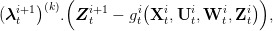It can be decomposed as

λ_tⁱ⁺¹^(k).Z_tⁱ⁺¹: term pertaining to dam i + 1.
−λ_tⁱ⁺¹^(k).g_tⁱX_tⁱ,U_tⁱ,W_tⁱ,Z_tⁱ: term pertaining to dam i.

Finally, the following term is added to the cost of dam i

( ) ( ) ( ) λit (k).Zit − λi+t1 (k).git Xit,Uit,Wit, Zit .

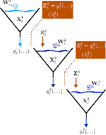
The main idea of the price decomposition of the problem is to see Z_tⁱ as an independent control variable as shown in ﬁgures 3. As U_tⁱ does, Z_tⁱ has to observe the (3) constraint.


(a)	(b)

Figure 3: (a): Whole Problem (b): Decomposed Problem

Then, we would like to solve the resulting N independent one-dam subproblems by DP¹ ,

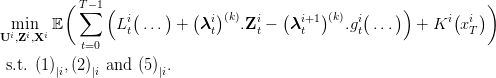( T∑ −1( ( ) ( )(k) ( )(k) ( ) ) ( )) min 𝔼 Lit ... + λit .Zit − λi+t1 .git ... + Ki xiT Ui,Zi,Xi t=0 s.t. (1) ,(2) and (5) . |i |i |i

(6)

But, the presence of the random variables λ_tⁱ_{t=0,…,T−1}^(k) prevents to use dynamic programming in a straightforward manner since the random variables λ_tⁱ are not independent over time. The idea of DADP is to replace the multipliers λ_tⁱ^(k) by their conditional expectations w.r.t. chosen information variable Y_tⁱ, namely

(ˆi)(k) (( i)(k) || i) λt := 𝔼 λt Y t .

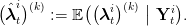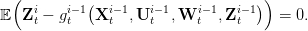
Note that this is equivalent to replace the (3) constraint by 𝔼Z_tⁱ − g_tⁱ⁻¹(…) |
|| Y_tⁱ = 0. In practice, Y_tⁱ is a short-memory process that will enter the state variables of the subproblems. In the sequel we will consider that Y_tⁱ ≡ const, so that _tⁱ^(k) := 𝔼λ_tⁱ^(k).

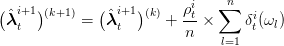
Thus, the Uzawa algorithm reads:

initialization: choose initial values for the multipliers _tⁱ⁽⁰⁾ for all i and t,
minimization: solve N independent one dimensional subproblems by dynamic programming,
$( ) T∑−1 ( i( ) ( i)(k) i ( i+1)(k) i( )) i( i ) miini i𝔼 Lt ... + λ t .Zt − λt .gt ... + K xT U ,Z,X t=0 s.t. (1) ,(2) and (5) . |i |i |i$

coordination: update the multipliers by a gradient step as follows:

simulation: apply the current strategy on a sample of n noise trajectories ω_l, to get n realizations of the random variables (g_tⁱ(…))^(k+1)(ω_l) by time step, compute all discrepancies (δ_tⁱ)(ω_l) in the coupling constraints given by:

i i i− 1( i−1 i−1 i−1 i− 1) (δt)(ωl) := Zt(ωl) − gt X t ,U t ,W t ,Z t (ωl),

gradient step: update the multipliers by taking the average of the discrepancies (δ_tⁱ)(ω_l)
$i ∑n (ˆλi+1)(k+1) = (ˆλi+1) (k) + ρt× δi(ω ) t t n t l l=1$

stopping condition: go to step (2) until convergence of the algorithm.

Question 5 Run the script job.sce to see iterations of the DADP algorithm solving the three cascade interconnected dams problem. You should observe the multipliers expected values and the dual costs converging in about three thousand iterations. At the end of iterations you can obtain the optimal multipliers expected values using the function dadp_get_lambda(). Use this function to store this values in matrix OPT_LAMBDA by calling OPT_LAMBDA=dadp_get_lambda().

Figure 4: Uzawa algorithm

Question 6 Have a look at the Uzawa algorithm ﬁgure Figure 4. Implement your own gradient step process and make the gradient step size values vary to see how it aﬀects the convergence of the algorithm. You can use the following program skeleton.

  exec loader.sce
  nspsoc('load_data');
  l1=[];l2=[];cost=[],costa=[],costaa=[],costab=[];
  dadp_set_gstep([1*ones(11,1),0.1*ones(11,1)]);
  for i=1:200
    dadp_minimization_step(); // DP for each dam given lambdas
    // now you should update the lambdas using the following functions
    // dadp_coordination(): computes the lambda gradients that you can then
    // obtain with dadp_get_dlambda();
    // then dadp_get_gstepsize() returns the gradient stepsizes.
    // you can get or set the current values of lambda with
    // L=dadp_get_lambda();
    // or
    // dadp_set_lambda(L);
  end

Question 7 Write your own dadp_coordination() function using the following code skeleton and then compare your code to the reference one.

  function [dl,dc]=dadp_coordination1()
    ndams = dadp_ndams();
    T = dadp_horizon();
    Nu = dadp_n_uzawa_scenarios();
    // dc: used to store the dual cost
    // dl: used to accumulate the average gradients it should be of size
    // zeros(2,T-1);
    for ksimul=0:Nu-1
      //  dadp_x0(); // gives the initial stocks
      for t=0:T-2
        // dadp_get_noise(ksimul,t); // get the intakes and price
        // [xp,u,g,costs]=dadp_dynamics(ksimul,t,x,w);
        ...
      end
      // dadp_final_cost(x); // returns the final cost for each dam
    end
    dc =- dc /Nu; // average
    dl = dl/Nu; // average
  endfunction

Question 8 You can change the previous function dadp_coordination1 in order to get the deviations from the coupling constraints trajectories at the optimal multipliers expected values. Compute these values when at the optimal multipliers expected values that you have stored before.

The approximation Y_tⁱ ≡ const is a relaxation of the problem (as the constraint is loosened). Thus, the strategies that we derive may not be feasible, even if the algorithm converges: we have to design a method to go back to a feasible strategy.

3.2 A heuristic to construct an admissible solution

Once the algorithm has converged we have feedbacks laws that verify the constraint

( ) 𝔼 Zi− gi− 1(Xi −1,Ui −1,Wi −1,Zi− 1) = 0. t t t t t t

But, this means that the physical constraint Z_tⁱ = g_tⁱ⁻¹…a.s. is not veriﬁed. Consequently one has to deﬁne an heuristic to turn this strategies into an admissible one.

We ﬁrst note that the optimal control to apply along a given noise trajectory may be computed using the Bellman function. The way to do this is the following: suppose that you have the three dimension DP-computed Bellman function

For every scenario
  For t=0:1:T-1
    get the current state and the inflow value for every dam;
    set a variable opt_cost to infinity;
    For u_i=0:4:40 (a loop a dam, three loops here thus)
      set the corresponding instant cost to a variable cost;
      apply the dynamic to get the reached states;
      add the reached states t+1 Bellman function value to cost;
      If cost < opt_cost then
       opt_cost=cost and set the u_i values to a vector opt_u;
    apply the dynamics with u=opt_u and collect the new current states;

Question 9 Use the simulation part of the previous coordination function to implement the simulation using the Bellman function you get by DP and compare it to the dp_simu() results.

We don’t have the three dimension Bellman function but we can construct an approximate Bellman’s value function for the global problem as the sum of the Bellman’s value function of each subproblem. Consequently we obtain a global admissible strategy by doing a one time step optimization of the global problem. More precisely if we write V _tⁱ(x_tⁱ) the Bellman’s function obtained for subproblem i when the DADP algorithm has converged, we deﬁne V˜t (x_t) = ∑ _i=1^NV _tⁱ(x_tⁱ⁻¹,x_tⁱ,x_tⁱ⁺¹), with the convention that¡ x₀^t = 0. Then the control we choose at time t when the cascade of dams is in the state x_t and the w_t is observed is the optimum of

∑N ( ) min Li xi,ui,wi + V˜t+1(f (xt,ut,wt )). ut i=1 t t t t

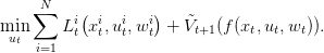This problem is global on the cascade but only done on one time-step, so numerically tractable.

Question 10 Apply the heuristic to the optimal strategy we computed using dadp_admissible() and simulate with [cost, stocks, controls]=dadp_simv(). Use the function which checked for the feasibility of the DADP computed strategy to see that the strategy is now feasible. Compare the results with those we get by the application of the exact optimal strategy.

A decomposition-coordination method for the cascade interconnected dams problem

Contents