Please launch software Scilab on your computer. To install Scilab, please consulthttp://www.scilab.org.
On this Internet page, you will find Scilab instructions lines starting with -->. Youwill copy them (or paste them by copy-paste) in the Scilab window to see how theyare executed. Beware not to copy the prompt -->.
Every line starting with //is a line of comments and is not executed byScilab.
1 Scalars, vectors, matrices
scalars
To begin, just type “x=8” in the Scilab window.
-->x=8
// Scilab affects the value 8 to the variable x
-->5
// Scilab affects the value 5 to the variable ans
// (for answer)
-->ans^2
// ans to the power 2 gives 25
-->abs(-5)
// absolute value
-->m=10^6
-->sqrt(m)
// square root
-->y=%e
-->log(y)
// %e is the constant e
-->sin(%pi)
// %pi is the constant pi
-->1+%eps
// %eps is the precision
complex numbers
-->%i
-->%i^2
-->x=3-4*%i
-->abs(x)
// modulus
vectors
-->v=[3.8,-4,%pi/6]
-->size(v)
// dimensions of v : 1 row and 3 columns
-->w=v'
// transposition
-->x=[1,2]; y=[3,4,5]
-->z=[x,y];
// construction of a vector by assembling blocks
-->t=[4:9]
// vector made of reals ranging from 4 to 9 by step 1
// (implicit set: 1 by defect)
-->t=[4:1:9]
// the same but with explicit step
-->t=[0:0.1:1]
// vector made of reals ranging from 0 to 1 by step 0.1
-->t=[0:0.1:%pi]
-->u=%e*[1:2:8]'
-->size(u)
-->s=ones(u)
// s is a vector with the same dimension as u
// all the elements of s are equal to 1
-->zeros(u)
// vector with the same dimension as u
// all the elements are equal to 0
-->t=rand(1,5)
// t is a vector with 1 row and 5 columns
// whose elements are randomly chosen in the interval [0,1]
-->v=rand(s)
// v is a vector with the same dimension as s
// whose elements are randomly chosen in the interval [0,1]
matrices
-->[1,2;3,4]
-->[11,12,13,14,15,16,17,18,19;21,22,23,24,25,...
-->26,27,28,29;31,32,33,34,35,36,37,38,39]
// when an instruction is too long to hold in a single line
// interrupt it by ... before changing line
-->diag([5 4 3])
// diagonal matrix
-->eye(6,6)
// matrix full of 0 except for the diagonal filled with 1
-->B=eye(6,7)
-->A=ones(3,7)
-->C=[A;(-6)*B]
-->D=zeros(2,5)
-->E=rand(D)
-->rand(2,5)
Question 1
Build a matrix with 4 rows and 9 columns with 1 on the first row and 0 everywhereelse. Use the above examples to build it by blocks.
Build a matrix with 3 rows and 5 columns: the first column is made of 2, the second ofintegers ranging from 1 to 3, and the rest is made of -1.
2 Usual vectorial operations
functions (with vector arguments)
-->u=2*%pi*rand()
// u is randomly chosen in [0,2*pi]
-->w=[cos(u) sin(u)]
-->norm(w)
// the euclidian norm of w is 1 since cos^2(u)+sin^2(u) = 1
-->norm(w,1)
// the 1-norm of w is |cos(u)|+|sin(u)|
-->t=2*%pi*rand(1,6)
-->v=sin(t)
-->maxi(v)
// the maximum value of the elements of v
-->[m,k]=maxi(v)
// the maximum value of the elements of v is m
// this maximum value m is reached at elements with index k : m=v(k)
-->[m,k]=mini(v)
-->sign(v)
// signe 1 (+) ou -1 (-) and sign(0)=0
logical operations
-->1==0
// is 1 equal to 0? the answer is F (false)
-->1~=0
// is 1 different from 0? the answer is T (true)
-->1==0 & 1~=0
// and: the answer is F (false)
-->1==0 | 1~=0
// or: the answer is T (true)
-->t=[0:%pi/2:2*%pi]
-->v=sin(t)
-->v>0
// returns a vector whose elements are T (true) or F (false)
// T if the correspond element is >0, F if not
-->v>=0
-->v(v>=0)
// extracts the nonnegative elements of v
// this vector may have less elements than v
-->bool2s(v>=0)
// converts the T and F in 1 and 0
addition
-->w=1:9
-->sum(w)
// gives the sum of all elements de w
-->cumsum(w)
// this is a vector consisting of the sequence of cumulated sums
-->A=rand(2,3)
-->B=sin(A)
-->A+B
-->G=[ones(1,4); 2*ones(1,4)]
-->sum(G,'c')
// sums the rows of the matrix G:
// the resulting object is a column vector ('c' for column)
-->sum(G,'r')
// sums the columns of the matrix G:
// the resulting object is a row vector ('r' for row)
-->D=rand(3,3)
-->expm(D)
// matrix exponential: EXPM(d)=I +D + D^2/2! + D^3/3! + ...
-->exp(D)
// beware: exp(D) is a matrix in which each element is the
// exponential of the corresponding element of D
extracting elements from a vector
-->w=1:2:9
-->w(2)
-->w($) // last element
-->w($-1) // before-last element
extracting submatrices
-->E=[11:19;21:29;31:39;41:49;51:59;61:69]
-->E(1,1) // the element of row 1 column 1
-->E(3,4) // the element of row 3 column 4
-->E(1,:) // the whole row 1
-->E(:,5) // the whole column 5
-->E(2:4,:)
// the submatrix made of rows ranging from 2 to 4
-->E(2:3,7:9)
// the submatrix made of elements belonging both to
// rows ranging from 2 to 3 and to columns ranging from 7 to 9
-->E([1,3,5],[2,4,6,8])
// the submatrix made of elements belonging both to
// rows ranging 1 3 5 and to columns 2 4 6 8
-->E(:,$) // last column
-->E(:,$-1) // before-last column
-->E(2:$,:)
// the submatrix made of rows ranging from 2 to the last row
-->E(2:($-1),:)
// the submatrix made of rows ranging from 2 to the before-last row
other functions
-->a=int(20*rand(1,10))
// integer part
-->[sa,ia]=sort(a)
// sorting: sa is the sorted vector, ia the corresponding indexes
3 Term by term vectorial operations
term by term multiplication
-->x=[1 2 3]
-->x.*x
-->y=[-6 12 8]
-->x.*y
-->A=rand(2,3);
-->B=ones(A);
-->A.*B
term by term division
-->x=[1 2 3]
-->y=1 ./x
// a space follows the 1, for if not 1. would be interpreted as 1.0 and
// the operation would be / (linear system resolution)
-->x.*y
-->A=rand(2,3);
-->B=rand(A);
-->A./B
term by term power
-->x=[1 2 3]
-->y=x.^2
-->z=x.^[5 10 -2]
-->A=rand(2,3);
-->A.^3
-->B=rand(A);
-->A.^B
Question 2
Build a matrix A=rand(5,3). This matrix has three columns: multiply the first columnby 5, the second by 2 and the last by 7; use only the following Scilab operations *, .*and ones.
4 2D graphics
For planar graphs, you have Scilab macros plot (elementary) and plot2d (with many
options).
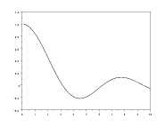
plot
-->x=0.1:0.1:10;
-->y=sin(x)./x;
-->plot(x,y)
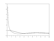
plot2d
Execute the instruction help plot2d to have information about the many options of
plot2d.
-->x=0.1:0.1:10;
-->y=sin(x)./x;
-->z=cos(x)./x;
-->xbasc();
// erase the graphic content of the window
-->plot2d(x,y);plot2d(x,z)
// both graphics are superposed
-->xbasc();plot2d([x ; x]',[y ; z]')
// the same, but both graphics are drawn each with its own color
// [x ; x]' is a matrix with 2 colonnes, as is [y ; z]'
// so that two curves are drawn
-->xbasc();plot2d([x' x'],[y' z'])
// gives the same result since [x ; x]' coincides with [x' x']
// and [y' z'] avec [y ; z]'
--> xset("window",2)
// window 2 is now active and future graphic instructions will
// appear in this window
--> plot2d(x,y)
--> xset("window",3) ; plot2d(x,z)
--> xdel(0)
// deletes the window 0
--> xdel(2:3);
// deletes the windows from 2 to 3
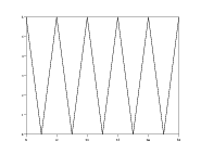
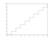
-->y=[6:-1:0,1:5] ; x =[y,y,y,y,y];
-->xbasc();plot2d(0:60,[x,6]);
// a simple graphic
-->xbasc();plot2d(0:60,[x,6],strf="011",rect=[0,0,60,6])
// the frame is fixed by rect =[xmin,ymin,xmax,ymax]
-->xbasc();plot2d(0:60,[x,6],strf="011",rect=[0,0,60,6],...
nax=[0,5,0,6])
// when an instruction is too long to hold in a single line
// interrupt it by ... before changing line
// nax=[0,5,0,6] fixes divisions and subdivisions on the axes
// execute instruction help plot2d to see all the options
plot2d2
-->x=1:10;
-->xbasc();plot2d2(x,x);
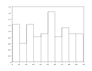
histogrammes
-->histplot(10,r)
// draws the histogram of 100 reals randomly chosen in [0,1]
-->xbasc()
-->histplot(0:0.2:1,r)
// the same but in choosing the sizes of the classes
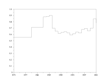
Question 3Plot the years in abcissa and the price of gasoline (euros of 2001) in ordinates. Takecare that the ordinates graph ranges from 0 to 1 euro.
annees=[1973 1979 1983:2001]
// only some years are available
prix_gazole_EC2001=[0.557 0.715 0.879 0.885 0.902 0.699 0.652 0.618 ...
0.633 0.643 0.627 0.592 0.614 0.638 0.624 0.681 0.697 0.658 0.702 0.848 0.783]
// price of gasoline (euros of 2001)
5 Programming
Scilab is an interpreted language, where the transmission of the arguments is made by value, even
for the objects of matrix type. It is thus recommended to avoid the loops, as they can prove
ineffective in term of computation time. For that purpose, it is better, if possible, to make use of
the vectorial operators who perform the same operations.
We recommend to use a text editor (Emacs), to open a file (for instancefile_name.sce), to write the code lines and to execute them inside Scilab with theinstruction exec("file_name.sce").
condition if
p=0.4
y=rand(1)
if y< p then x=1;
elseif y>= p then x=0;
end
x
boucles while
p=0.2
y=rand(1);
compteur=1;
while y >=p do compteur=compteur+1; y=rand(1); end
compteur
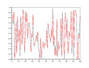
boucles for
N=500;
y=rand(1,N)-0.5*ones(1,N);
x=sign(y);
for i=2:N,x(i)=x(i-1)+x(i);end;
xbasc();plot2d(1:N,x)
x1=cumsum(sign(y));
norm(x1-x)
6 Scilab functions
One may define a Scilab function interactively. However, it is more practical andflexible to write the Scilab code in a file with a text editor. One can mixScilabinstructions Scilab and functions definitions in a same file, named with theextension .sce.
The beginning of a Scilab function is function [<arguments de retour>]=<nom>(<arguments d'entrée>) and the code ends with the keyword endfunction.
function [y]=densite(x), y=1 ./(%pi*sqrt(x.*(1-x))), endfunction;
A Scilab function in Scilab may have several arguments, scalars or vectors.
function [y]=Gauss(x,mu,sigma)
// mu and sigma are scalars
// x may be a vector of any dimensions
y=1 ./(sigma*sqrt(2*%pi))*exp(-((x-mu)/sigma).^2/2)
endfunction;
function [Y]=Normal(X,Mu,Sigma)
// Mu is a row vector with dimensions [1,dim]
// Sigma is a positive symmetric matrix with dimensions [dim,dim]
// x may only be a vector with dimensions [1,dim]
[lhs,dim]=size(Mu)
Y=1/ sqrt( (2*%pi)^dim * det(Sigma) ) * ...
exp(- (X-Mu)*inv(Sigma)*(X-Mu)' / 2 )
endfunction;
A Scilab function in Scilab may have several outputs.
function [H,plus] = Heavyside_plus(x)
// Heavyside function
H = maxi(sign(x),0);
// Heavyside(0)=1
plus=maxi(x,0)
// Function +
endfunction
[H,plus] = Heavyside_plus(-1:0.2:1)
function [x]=permutation_lent(n)
// permutation aléatoire de {1,...,n}
// version avec des boucles
x=ones(1,n);
for i=2:n,k=0;
for j=1:1+int(rand(1)*(n-i+2));k=k+1;
while x(k)>1 do
k=k+1;
end;
end;
x(k)=i;
end;
endfunction
function [x]=permutation_rapide(n)
// permutation aléatoire de {1,...,n}
x=grand(1,'prm',[1:n]')
endfunction
// loading of function permutation_lent :
-->exec("nom_du_fichier.sce")
// the function is now loaded
-->permutation_lent
// call of function permutation_lent
-->permutation_lent(100)
7 Simulation of dynamic systems in discrete time
We consider the discrete time dynamics system in :
(1)
starting from initial state at time
(2)
Knowing function and , we are able to compute the whole sequence
solution of the problem.
7.1 Population dynamics in ecology
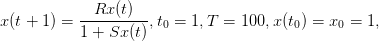
Consider the population dynamics
with parameters and .
t0=1;x0=1;
x(t0)=x0; T=100; R=1.2; S=0.02;
function y=f(t,x)
y=R*x./(1+S*x)
endfunction
for (t=t0:1:T)
x(t+1)=f(t,x(t));
end;
plot2d(t0:T+1,x(t0:T+1))
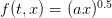
Question 5Change the population dynamics withwhere.Compare the behavior of the solutions.
7.2 Carbon cycle
Consider the carbon cycle
starting from initial conditions (ppm) at year with time horizon
. The parameters are , preindustrial concentration ,
removal rate . It is assumed that the ”business as usual” CO emissions path
is
with the emissions growth set to and initial emissions to
(GtC).
function y=EBAU(t)
y=E_BAU*(1+g)^(t-t0);
endfunction
function y=f(t,M)
y=M+alpha*EBAU(t)*(1-a)-delta*(M-M_infty);
endfunction
x(t0)=M_0;
for (t=t0:1:T)
x(t+1)=f(t,x(t));
end;
plot2d(t0:T+1,x(t0:T+1),rect=[t0,0,T+1,1000])
Question 6Change the mitigation rate() to compare the behavior of theconcentrations profile.
7.3 An ecosystem
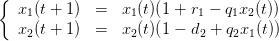
We consider two populations interacting within a trophic web. The dynamics based on
a Lotka-Volterra form is characterized by
(3)
where is the intrinsic growth of prey while is the intrinsic decrease of
predator. Parameters are related to the catchability and efficiency of trophic
relations.


 ).
).
 :
:

 at time

 and
and  , we are able to compute the whole sequence
 solution of the problem.
 and
and  .
.
 where
where  .
Compare the behavior of the solutions
.
Compare the behavior of the solutions  .
.

 (ppm) at year
  with time horizon
 . The parameters are
  , preindustrial concentration
  ,
removal rate
,
removal rate  . It is assumed that the ”business as usual” CO
 emissions path
is
emissions path
is

 and initial emissions to
 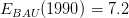 (GtC).
 (
(![a ∈ [0, 1]](english_intro_scilab34x.png) ) to compare the behavior of the
concentrations profile
) to compare the behavior of the
concentrations profile  .
.
 interacting within a trophic web. The dynamics based on
a Lotka-Volterra form is characterized by
interacting within a trophic web. The dynamics based on
a Lotka-Volterra form is characterized by
 is the intrinsic growth of prey while
  is the intrinsic decrease of
predator. Parameters
is the intrinsic decrease of
predator. Parameters  are related to the catchability and efficiency of trophic
relations.
are related to the catchability and efficiency of trophic
relations.
 or
or  to compare the behavior of the populations
 .
.


