Fermer X

Contents

Let time t be measured in discrete units (such as years). Let B(t) denote the biomass of a population at time t (beginning of time interval [t,t + 1[). We consider the so called Schaefer model

B (t + 1) = Biol(B(t)) − h(t),   0 ≤ h(t) ≤ Biol(B (t))
(1)

where Biol is the population dynamics and h(t) is the harvesting. Notice that, in the time interval [t,t + 1[, growth of the stock occurs first, followed by harvesting1 .

The sustainable yield he = Sust(Be) solves Be = Biol(Be) he, which gives:

Sust (B ) := Biol(B ) − B.
(2)

The carrying capacity of the habitat is the level K > 0 of positive biomass such that Biol(K) = K, that is Sust(K) = 0.

The maximum sustainable yield hmse and the corresponding maximum sustainable equilibrium Bmse are

hmse := sup [Biol(B ) − B ] and  Bmse := arg max [Biol(B ) − B ].
       B ≥0                                 B≥0
(3)

From [1, p. 258] and numerical simulations, we shall consider the Pacific yellowfin tuna example as in Table 1.


Pacific yellowfin tuna


yearly intrinsic growth R = 2.25
carrying capacity K = 250 000 metric tons
catchability q = 0.0 000 385 per SFD
price p = 600 $ per metric ton
cost c = 2 500 $ per SFD


Table 1: Pacific yellowfin tuna data for a discrete time logistic model (adapted from [1, p. 258]). SFD: standard fishing day.

1 The Beverton-Holt model

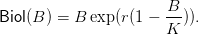
The Beverton-Holt model is characterized by the discrete time dynamics mapping
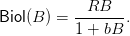
          --RB---
Biol(B ) = 1 + bB .
(4)

We have

           --                  --
        (√ R − 1)2           √ R −  1             R  − 1
hmse =  ----------,  Bmse  = --------  and   K  = ------.
            b                   b                    b
(5)

Question 1 Use the data in Table 1 to compute b in (4). Give the maximum sustainable biomass Bmse and the maximum sustainable yield hmse as in (5).

  
  R_tuna = 2.25 ;
  K_tuna = 250000 ; // metric tons
  
  // BEVERTON-HOLT DYNAMICS
  R_BH = R_tuna ;
  b_BH = (R_BH-1) / K_tuna ;
  
  function [y]=Beverton(B)
  y=(R_BH*B)./(1 + b_BH*B) ;
  y=maxi(0,y) ;
  endfunction;
  
  // SUSTAINABLE YIELD MACRO
  function [SY]=sust_yield(dynamic,B), SY=dynamic(B)-B, endfunction;
  
  
  // MAXIMUM SUSTAINABLE EQUILIBRIUM
  B_MSE = (sqrt(R_BH) - 1)/b_BH ;
  // maximum sustainable yield
  h_MSE = sust_yield(Beverton,B_MSE) ;
  // maximum sustainable yield
  

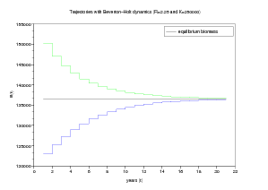
Question 2 Select one biomass level Be between the maximum sustainable biomass Bmse and the carrying capacity K. Compute the corresponding sustainable yield he.

Draw the corresponding steady trajectory of the Schaefer model (1) with the Beverton-Holt dynamics (4) and h(t) = he. Pick up two different initial conditions in the neighborhood of the equilibrium biomass Be. Draw the corresponding trajectories. Does the figure confirm or not the fact that the equilibrium biomass Be is attractive?

Recall that, for an equilibrium, being stable or attractive are unrelated notions.

Question 3 Does the figure confirm or not the fact that the equilibrium biomass Be is stable? Be specific in your justifications. What can you say about asymptotic stability of the equilibrium biomass Be?

  
  // SUSTAINABLE EQUILIBRIUM
  
  alpha=rand();
  Be= alpha*B_MSE + (1-alpha)*K_tuna ;
  // selection of one of many possible equilibria
  he=sust_yield(Beverton,Be) ;
  // corresponding sustainable yield
  
  
  function [y]=sequential(y0,time,f)
  [one,two]=size(Binit) ;
  y=zeros(one,prod(size(time))) ; // time is a vector t0, t0+1,...,T
  // vector will contain the trajectories y(1),...,y(T-t0+1)
  // for different initial conditions
  for k=1:one
  y(k,1)=y0(k);
  // initialization
  for s=time(1:($-1)) -time(1)+1
  // runs from 1 to T-t0+1
  y(k,s+1)=f(s,y(k,s));
  end ;
  end ;
  endfunction
  
  
  // STATE TRAJECTORY UNDER DYNAMICS
  
  function [y]=Beverton_e(t,B)
  y=Beverton(B) - he ;
  y=maxi(0,y) ;
  endfunction
  // Beverton-Holt dynamics with harvesting at equilibrium (Be,he)
  
  T=20;
  years=1:(T+1);
  
  xset("window",31); xbasc(31);
  Binit=Be;
  Bt=sequential(Binit,years,Beverton_e);
  plot2d2(years',Bt',1);
  //
  Binit=0.9*Be ;
  Bt=sequential(Binit,years,Beverton_e);
  plot2d2(years',Bt',2);
  //
  Binit=1.1*Be;
  // It seems there is a bug with the previous version of 'sequential'
  Bt=sequential(Binit,years,Beverton_e);
  plot2d2(years',Bt',3);
  //
  xtitle('Trajectories with Beverton-Holt dynamics (R=' +string(R_tuna)...
  +' and K=' +string(K_tuna) +')', 'years (t)','B(t)')
  legends(['equilibrium biomass'],[1],'ur')
  

PICT

Figure 1: Pacific yellowfin tuna biomass trajectories with Beverton-Holt dynamics

Question 4 Find an equilibrium state Be which is not attractive. Illustrate that Be is not attractive with some trajectories. What can you say about asymptotic stability of the equilibrium biomass Be?

With price p, catchability coefficient q and harvesting unitary costs c, the private property equilibrium (ppe) is the equilibrium solution (Bppe,hppe) = (Bppe,Sust(Bppe)) which maximizes the rent as follows:

                  ch
   max     [ph − ---].
B≥0,h=Sust(B )     qB
(6)

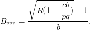
The common property equilibrium Bcpe makes the rent null and is given by

         c
Bcpe =  --.
        pq
(7)

Question 5 Study the stability around the two following equilibria:

  • common property equilibrium Bcpe,
  • private property equilibrium
            ∘ -------cb-
          R (1 +  --) − 1
B    =  ---------pq-----.
  ppe           b
    (8)

Compare your observations with the theoretical results.

  
  // Economic parameters
  c_tuna=2500; // unit cost of effort
  p_tuna=600; // market price
  q_tuna=0.0000385; // catchability
  
  c=c_tuna;
  p=p_tuna;
  q=q_tuna;
  
  B_PPE= ( sqrt( R_BH * (1 + (b_BH*c/(p*q)) ) ) - 1 ) / b_BH;
  // private property equilibrium
  
  B_CPE=c/(p*q) ;
  // common property equilibrium
  

2 The logistic model

The logistic model is characterized by the discrete time dynamics mapping
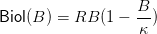
                   B
Biol(B ) = RB  (1 −  --)
                   κ
(9)

where R 1 and r = R 1 0 is the per capita rate of growth (for small populations), and κ is related to the carrying capacity K (which solves Biol(K) = K) by:

Biol(K ) = K  ⇐ ⇒  RK  (1 − K-) = K  ⇐⇒  κ =  --R---K ⇐ ⇒  K  =  R-−-1κ.
                           κ                 R − 1                R
(10)

We have

       (R-−--1)2    R-−--1                  R-−--1    K--
hmse =    4R    κ =    4  K   and   Bmse =   2R   κ =  2 .
(11)

Question 6 Adapt the previous Scilab code to the logistic model, and compare the results.

3 The Ricker model

The Ricker model is characterized by the discrete time dynamics mapping

                       B--
Biol(B ) = B exp (r(1 − K )).
(12)

Question 7 Adapt the previous Scilab code to the Ricker model, and compare the results. Try numerical procedures: type help fsolve to obtain information about Scilab solver.

References

[1]   M. Kot. Elements of Mathematical Ecology. Cambridge University Press, Cambridge, 2001.

L'École des Ponts ParisTech est membre fondateur de

L'École des Ponts ParisTech est certifiée 

ParisTech ParisEst ParisTech


Copyright 2014
École des Ponts ParisTech
All rights reserved