
| L'École des Ponts ParisTech est membre fondateur de |
L'École des Ponts ParisTech est certifiée |


|
|


We consider the discrete time dynamics system in ℝn:
 | (1) |
starting from initial state x0 ∈ ℝn at time t 0
 | (2) |
Knowing function f and (t0,x0), we are able to compute the whole sequence x(t0),x(t0 + 1),…,x(T) solution of the problem.
Consider the population dynamics
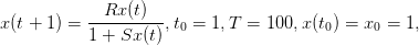
with parameters R = 1.2 and S = 0.02.
Question 1 Change the population dynamics with f(t,x) = (ax)0.5 where a = 10. Compare the behavior of the solutions x(t).
Consider the carbon cycle

starting from initial conditions M0 = 354 (ppm) at year t0 = 1990 with time horizon T = 100. The parameters are α = 0.471, preindustrial concentration M−∞ = 280, removal rate δ = 0.01. It is assumed that the ”business as usual” CO2 emissions path is

Question 2 Change the mitigation rate a (a ∈ [0, 1]) to compare the behavior of the concentrations profile M(t).
We consider two populations x1(t),x2(t) interacting within a trophic web. The dynamics based on a Lotka-Volterra form is characterized by
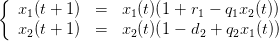 | (3) |
where r1 > 0 is the intrinsic growth of prey while d2 > 0 is the intrinsic decrease of predator. Parameters q1 > 0,q2 > 0 are related to the catchability and efficiency of trophic relations.
Question 3 Change parameters r,d or q to compare the behavior of the populations (x1(t),x2(t)).
| L'École des Ponts ParisTech est membre fondateur de |
L'École des Ponts ParisTech est certifiée |
|
|
|


