
| L'École des Ponts ParisTech est membre fondateur de |
L'École des Ponts ParisTech est certifiée |


|
|


We consider uncertainty modelled here by a set Ω, containing issues or scenarios. We present some classical measures attached to a scalar prospect (random variable) X : Ω → ℝ. Here, X represents a gain, a profit, a position, the value of a portfolio, etc., in a word a prospect while −X represents a loss.
When focusing on situations of risk, we shall suppose that Ω carries a probability ℙ (defined on a σ-field ℱ, so that (Ω,ℱ, ℙ) is a probability space). The expectation under probability ℙ is denoted by 𝔼.
The Value at Risk of a prospect X at level λ ∈]0, 1[ is
 | (1) |
Intuitively, saying that the V aR5% of a portfolio is 100 means that the loss −X will be larger than 100 with probability at most 5%. However, V aR5% does not inform on the size of the loss.
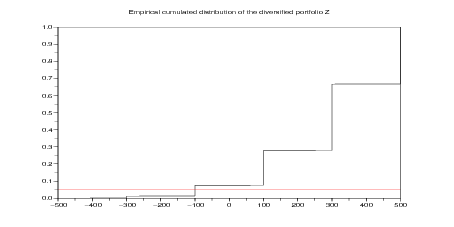
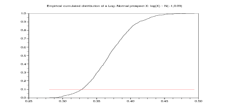
Question 1 Compute the Value at Risk at different levels (1 %, 5 %, 10 %) of a log-normal prospect. Draw the empirical cumulated distribution of a log-normal prospect.
A prospect X is said to be log-normal if X > 0 and log X ∼𝒩(μ,σ2).
Corporate bonds are sold at 95 $ and return 100 $ except in 2 % of cases where they lose all value. The prospect Xi provided is thus Xi = 100𝜀i − 95 ∈{5,−95}, where ℙ(𝜀i = 1) = 0.98 and ℙ(𝜀i = 0) = 0.02.
First, let us consider a fully concentrated portfolio C = 100X1, consisting of 100 units of the first bond. Second, let us consider a fully diversified portfolio D = 2 ∑ i=150X i, consisting of 2 units of each bond. The 𝜀1, …, 𝜀50 are supposed to be independent.
Question 2 Using the fact that V aR5%(𝜀1) = −1, and positive homogeneity and translation-invariance of V aR5%, compute V aR5%(X1), then V aR5%(C). Estimate V aR5%(D) by simulation. Conclude that withdrawing up to 500 $ from the fully concentrated portfolio C makes it acceptable, while you need to add a capital of at least 100 $ to the fully diversified portfolio D to make this latter acceptable.
The lottery  describes a hazard situation where
where all probabilities are greater than or equal to zero and sum up to one (100% chance).
Suppose that the outcomes  are scalar. Let us be given a utility function
 . The value of the lottery is the expectation of the utilities
  :
:

In a choice situation between two lotteries, the expected utility maximizer will select the one with the highest EU.
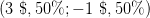
3 $ 50% -1 $50%
Lottery 1Y 1 000 000 $ 100% versus Lottery 1Z 1 000 000 $ 89% 0 $1% 5 000 000 $10%
Question 4 Which of the two above lotteries do you personnaly prefer? Load the function EU
following Question 3. Compute the expected utility of the lotteries  and
and
 for different utility functions:
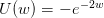
 , A > 0;
 , γ > 0, γ ⁄= 1, w > 0.
For each utility function, tell which lottery is prefered to the other one, and explain the reasons of your choice.
Lottery 2Y 1 000 000 $ 11% 0 $89% versus Lottery 2Z 5 000 000 $ 10% 0 $90%
Question 5 Same questions as in Question 5 for the lotteries
 and
and  .
.
In a bank questionnaire, the customer answers a series of questions ranging from 8 to 13. In question k, he is asked which lottery he prefers between a certain lottery LOTTERY_C(k) and a 50%-50% risky lottery LOTTERY_R(k).
Question 7 Load the function EU following Question 3. Test wether lottery LOTTERY_C(k)
is prefered to the 50%-50% risky lottery LOTTERY_R(k) for k = 8,…, 13, for the CARA utility
functions  , A > 0. Compute the Arrow-Pratt coefficient of absolute risk
aversion
, A > 0. Compute the Arrow-Pratt coefficient of absolute risk
aversion  . Select a proper range of values for the parameter A. How do you
explain what you observe when the parameter A varies?
. Select a proper range of values for the parameter A. How do you
explain what you observe when the parameter A varies?
Question 8 Same question for the CRRA utility functions  , γ > 0, γ ⁄= 1,
w > 0. Compute the Arrow-Pratt coefficient of relative risk aversion
, γ > 0, γ ⁄= 1,
w > 0. Compute the Arrow-Pratt coefficient of relative risk aversion  .
How do you explain what you observe when the parameter γ varies? Compare your results
with the one in the document Lettre à S. by the economist Laurent Denant-Boemont. Do you
agree with all his comments?
.
How do you explain what you observe when the parameter γ varies? Compare your results
with the one in the document Lettre à S. by the economist Laurent Denant-Boemont. Do you
agree with all his comments?
Question 9 Same question for the power-expo utility functions 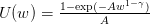 ,
1 > γ > 0, w > 0.
,
1 > γ > 0, w > 0.
(from (Gollier, 2001, p. 30)).
Suppose that you are a decision-maker who evaluates any prospect X by
 | (2) |
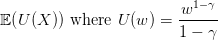
is a CRRA (constant relative risk aversion) utility function. The parameter γ > 0 is the relative risk aversion parameter.
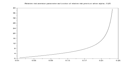
Consider the situation where you face the risk of gaining or losing a share 𝜃 of your wealth w0 with equal probability. The relative risk premium πγ(𝜃) is implicitely defined by
![1 1
U (w0(1 − π γ(𝜃 ))) = 𝔼 [U (w0X )] = -U (w0(1 − 𝜃)) + -U (w0 (1 + 𝜃))
2 2](risk_preferences22x.png) | (3) |
where X takes values 1 − 𝜃 and 1 + 𝜃 with equal probability 1∕2. The relative risk premium πγ(𝜃) is the share of your wealth that you are ready to pay to escape this risk.
Question 10 Give the formula for πγ(𝜃). For each 𝜃 =5 %, 15 %, 25 %, draw the curve giving the relative risk aversion parameter γ as a function of the relative risk premium. Fill in the second column of Table 2.4 with your relative risk premium and compute your relative risk aversion. Comment on what you observe.
//
| gaining or losing | fraction of your wealth | relative risk aversion |
| a share 𝜃 of your wealth | that you are ready to pay | parameter |
| (empirical risk premium) | ||
| 5 % | ||
| 15 % | ||
| 25 % | ||
(From (Kahneman and Tversky, 1979; Tversky and Kahneman, 1992))
Suppose that the prospect X takes a finite number of values
 | (4) |
with corresponding probabilities (nonnegative and summing up to one)
 | (5) |
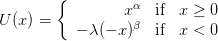
The evaluation of a prospect with null anchor x0 = 0 is given by
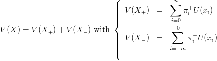 | (6) |
where U is a strictly increasing function such that U(0) = 0. When the anchor x0 is not necessarily zero, we evaluate the prospect by V (X − x0). The weighting functions for gains and losses are given by
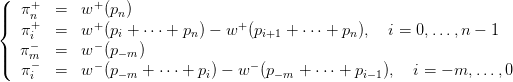 | (7) |
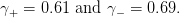
where w+ and w− are increasing functions satisfying w+(0) = w−(0) = 0 and w+(1) = w−(1) = 1. In (Tversky and Kahneman, 1992), one finds
 | (8) |
with experimental evidence consistent with
 | (9) |
For the weighting functions, (Tversky and Kahneman, 1992) proposes
![+ --------pγ+--------- − ---------pγ−--------
w (p) = γ+ γ+ 1∕γ+ and w (p) = γ− γ− 1∕γ−
[p + (1 − p) ] [p + (1 − p) ]](risk_preferences30x.png) | (10) |
with parameter values
 | (11) |
Cumulative Prospect Theory: Scilab code
//
Question 11 Same questions as in §2.2, but evaluating lotteries by CPT, with either zero anchor, or a positive one that you will choose.
Question 12 Same questions as in §3.4, but evaluating lotteries by CPT, with either zero anchor, or the value of the certain lottery.
Let us consider the problem in Sect. 2. Suppose that you face the risk of gaining or losing a share
𝜃 of your wealth x0 with equal probability. The relative risk premium πCPT (𝜃) is the share of your
wealth that you are ready to pay to escape this risk. Expressing indifference between this risk and
the certain prospect x0 1 − 𝜃
1 − 𝜃 gives:
 | (12) |
Notice that (8) with α = β implies that the evaluation of a prospect with respect to an anchor is invariant with respect to a positive scaling factor (of both the prospect and the anchor). We thus write the above equation with x0 = 1, to obtain:
 | (13) |
In the end
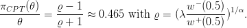 | (14) |
| gaining or losing a share 𝜃 of your wealth | CPT relative risk premium |
| 5 % | 2.3 % |
| 15 % | 7 % |
| 25 % | 11.6 % |
(From (Pfiffelmann and Roger, 2005))
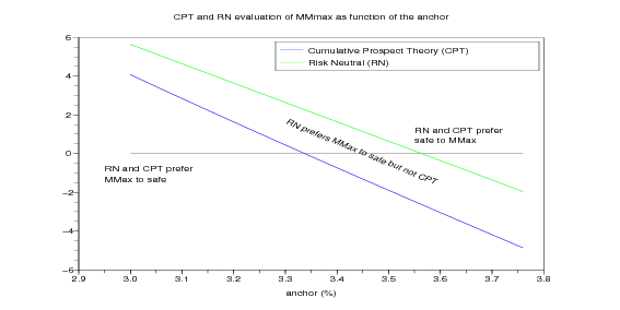
The compte d’épargne MMmax was launched in November 2003 by Mutuelles du Mans. This financial product returns 2.5 % for sure every year and, when lucky, additional 5 %, 10 % or 20 % (see details in the Scilab code below). We want to test its success to the public by comparison with a safe product returning a fixed rate every year (anchor).
Question 13 The values for MMmax are given below. Show that its mean return is slightly more than 3.5% Draw the evaluation of this product as function of the anchor for an investor evaluating prospects according to Cumulative Prospect Theory (CPT investor, in short). Observe that any safe product with return more than 3.3% is prefered to the risky MMmax. Conclude that a CPT investor is less encline to invest in MMmax than in safe product, compared to a risk-neutral investor.
//
Rudiger Frey and Alexander J. McNeil. Var and expected shortfall in portfolios of dependent credit risks: Conceptual and practical insights. Journal of Banking and Finance, 26:1317–1334, 2002.
C. Gollier. The Economics of Risk and Time. MIT Press, Cambridge, 2001.
Daniel Kahneman and Amos Tversky. Prospect theory: An analysis of decision under risk. Econometrica, 47(2):263–292, 1979.
Marie Pfiffelmann and Patrick Roger. Les comptes d’épargne associés à des loteries: approche comportementale et étude de cas. Banque & Marchés, septembre 2005.
Amos Tversky and Daniel Kahneman. Advances in prospect theory: Cumulative representation of uncertainty. Journal of Risk and Uncertainty, 5(4):297–323, October 1992.
| L'École des Ponts ParisTech est membre fondateur de |
L'École des Ponts ParisTech est certifiée |
|
|
|


