The newsvendor problem

Michel De Lara
(last modiﬁcation date: February 22, 2019)

Version pdf de ce document
Version sans bandeaux

1 The newsvendor problem (integer formulation)
2 The newsvendor problem (continuous formulation)
3 The newsvendor problem with risk (continuous formulation)
4 The newsvendor problem with backorder (continuous formulation)

1 The newsvendor problem (integer formulation)
1.1 The demand distribution is uniform
1.2 The demand distribution is a mixture of two truncated Poisson distributions
1.3 The demand distribution is triangular
2 The newsvendor problem (continuous formulation)
3 The newsvendor problem with risk (continuous formulation)
4 The newsvendor problem with backorder (continuous formulation)

1 The newsvendor problem (integer formulation)

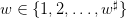
Each morning, the newsvendor must decide how many copies u ∈{1, 2,…,u^♯} of the day’s paper to order. The variable u is called control.
During the day, the newsvendor will meet an unknown demand $w ∈ {1,2,...,w ♯}$ . The variable w is called uncertainty.
The newsvendor faces an economic tradeoﬀ:
- he pays the unitary purchasing cost c per copy, when he orders stock;
- he sells a copy at price p;
- if he remains with an unsold copy, it is worthless (perishable good).
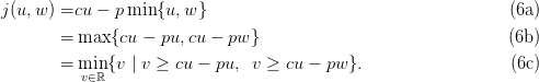
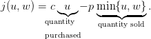
Therefore, the newsvendor’s costs are (where w ∈{1, 2,…,w^♯} is a possible value of the demand)
$j(u,w ) = c◟◝u◜◞ − pm◟in-{◝u◜,w-}◞. quantity quantity sold purchased$ (1)

The newsvendor’s payoﬀ is −j(u,w).

Now, we introduce a random variable W, where W : Ω →{1, 2,…,w^♯}. Here, Ω is an underlying probability space, equipped with a probability ℙ. We suppose that the newsvendor knows the probability distribution ℙ_W of the demand W.

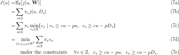
Thus equipped, we consider the stochastic optimization problem of expected costs minimization:

min J(u) = 𝔼 [j(u, W )]. u∈{1,2,...,u♯} ℙ

(2)

  // demand
  wsharp=100;// no larger, else the Poisson distribution cannot be computed
  wflat=1;
  demand=[wflat:wsharp];

  // control
  control=[demand,1+demand($)];

  // Criterion / costs
  cc=1;pp=10*cc;
  // cc=1 ; pp=1.1*cc ;
  // avoid that cc/pp is the inverse of an integer
  // when the distribution of demand is uniform
  costs=cc*control'*ones(demand)-pp*mini(ones(control')*demand,control'*ones(demand));
  // one row by control, one column by demand

We will consider diﬀerent demand distributions.

1.1 The demand distribution is uniform

First, we suppose that the demand distribution ℙ_W is uniform as follows.

probab=ones(demand);
probab=probab/sum(probab);

Question 1

a)

[1] Draw a histogram of the random demand W.

b)

[1+1] In the scilab code above, what does the matrix costs represent? (What do you ﬁnd at the intersection of a row and of a column?) Explain in detail why we have that criterion = probab*costs’ is a row vector made of the values of $J (u) = 𝔼ℙ[j(u,W )]$ for u ∈{1, 2,…,u^♯}?

c)

[1+1] Draw the mapping u ∈ {1, 2,…,u^♯}

J(u). Thanks to the scicoslab macro mini (that provides the minimum and the argmin index of a vector), give the numerical value of the decision u^⋆ (optimal order) that minimizes u

J(u).

d)

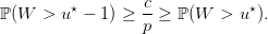
[1+1] What does the vector decumprobab=1-cumsum(probab) represent? Explain your answer. Check that, in agreement with the theory, we numerically have that

ℙ(W > u⋆ − 1) ≥ c-≥ ℙ (W > u⋆). p

e)

[2+1] For a given value of u, explain why the random variable $j (u, W )$ can at most take the values ${j(u,1),...,j(u,u − 1),j(u,u )}$ . Give, for each of the u elements of this list, the corresponding probability that $j(u,W )$ takes this value in the list. In the end, you will provide an expression of the probability distribution of $j(u,W )$ , using probab and decumprobab.

f)

[1+2] Draw histograms of the probability distribution of the random payoﬀ (the opposite of the costs) $− j(u, W )$ for u = u^⋆ (the optimal decision) and for u = 𝔼_ℙ[W] (the naive deterministic solution consisting in ordering the mean demand 𝔼_ℙ[W]). Draw the two histograms on the same picture, so that they have the same scale. Comment on the diﬀerences between the two histograms.

g)

[1+1+1+2] The vector grand(365,"markov",ones(probab’)*probab,1) represents a sequence of realizations of 365 i.i.d. random variables having the same distribution than the demand W. Simulate and draw the trajectory of the cumulated payoﬀs of the newsvendor during one year if, every day, he orders the optimal quantity u = u^⋆. Do the same for u = 𝔼_ℙ[W] and draw it on the same picture. In what sense does the the optimal decision u = u^⋆ does better than u = 𝔼_ℙ[W]? Justify in detail why the two trajectories are approximately straight lines; to what correspond the slopes?

h)

Now, we study if the results are robusts to changes in the the ratio between the unitary purchasing cost c and the selling price p.

1): [2] Take c < p with c ≈ p. Find the optimal decision u^⋆. Draw histograms of the probability distribution of the random payoﬀ $− j(u,W )$ for u = u^⋆ and for u = 𝔼_ℙ[W]. Simulate and draw trajectories of the corresponding cumulated payoﬀs.
2): [2] Same question with c << p.
3): [2] Discuss. In particular, how does the optimal solution u^⋆ vary with the ratio c∕p?

  //exec('newsvendor_data.sce');exec('newsvendor_uniform.sce');exec('newsvendor_main.sce')

  xset("window",1);clf();plot2d2(demand,probab)
  xtitle("Histogram of the demand")

  // Criterion / expected costs
  criterion=probab*costs';
  // a row vector
  xset("window",3);clf();plot2d2(control,criterion)
  xtitle("The expected costs as function of the decision")

  // Optimal decision
  [lhs,optcont]=mini(criterion);
  disp("The optimal decision is "+string(optcont))

  // Naive deterministic solution
  meandemand=probab*demand';
  disp("The expected demand is "+string(round(meandemand)))

  // Check that the optimal decision satisfies the optimality condition
  cumprobab=cumsum(probab);
  decumprobab=1-cumprobab;

  xset("window",4);clf();plot2d2(demand,decumprobab,rect = [demand(1)-1,0,demand($),1]);
  plot2d(demand,cc/pp*ones(decumprobab),style = 5);
  xtitle("The decumulative distribution of the demand")

  disp("Is it true that "+string(cc/pp)+" lies between "+string(decumprobab(optcont))+ ...
       " and "+string(decumprobab(optcont-1))+"?")

  NS=365;
  // simulated demands
  DD=grand(NS,'markov',ones(probab')*probab,1);

  time=[1:NS];

  xset("window",8);clf();
  plot2d2(time,cumsum(-costs(round(meandemand),DD)),style = 3);
  plot2d2(time,cumsum(-costs(optcont,DD)),style = 5);
  legends(["optimal solution "+string(optcont);
           "naive deterministic solution "+string(round(meandemand))],[5,3],"lr");
  xtitle("The cumulated payoffs as function of the number of days","time","payoff")


  xset("window",10);clf();
  uu=optcont;
  ss=5;
  plot2d2([costs(uu,[wflat:(uu-1)]),costs(uu,uu)], ...
          [probab([wflat:(uu-1)]),decumprobab(uu-1)],style = ss, ...
          rect = [mini(costs),0,maxi(costs),1]);
  //
  uu=round(meandemand);
  ss=3;
  plot2d2([costs(uu,[wflat:(uu-1)]),costs(uu,uu)], ...
          [probab([wflat:(uu-1)]),decumprobab(uu-1)],style = ss, ...
          rect = [mini(costs),0,maxi(costs),1]);
  //
  legends(["optimal solution "+string(optcont);
           "naive deterministic solution "+string(round(meandemand))],[5,3],"ur");
  xtitle("Histograms of the costs")

1.2 The demand distribution is a mixture of two truncated Poisson distributions

Second, we suppose that the demand distribution ℙ_W is a mixture of two truncated Poisson distributions as follows:

♭ w ♯w 1- ♭(λ-)-- 1- ♯(λ-)--- ♯ ℙW (w ) = ℙ(W = w) = 2 × k w! + 2 × k w! , ∀w ∈ {1,2,...,w }.

(3)

Question 2 [6] Same questions as in Question ?? when the demand W follows a mixture of two truncated Poisson distributions.

  // Poisson
  lambdaflat=wsharp/4;lambdasharp=3*wsharp/4;
  //
  probabflat=(lambdaflat .^demand) ./(factorial(demand));
  probabflat=probabflat/sum(probabflat);
  //
  probabsharp=(lambdasharp .^demand) ./(factorial(demand));
  probabsharp=probabsharp/sum(probabsharp);
  //
  probab=0.5*probabflat+0.5*probabsharp;

1.3 The demand distribution is triangular

Question 3 [6] Same questions as in Question 1 when the demand W follows a triangular distribution over {1, 2,…,w^♯}.

  // Triangular distribution
  lambda=floor(wflat+0.3*(wsharp-wflat));
  //
  probab=[cumsum(ones([wflat:lambda]))/sum(ones([wflat:lambda])), ...
          1-cumsum(ones([(lambda+1):wsharp]))/sum(ones([(lambda+1):wsharp]))];
  probab=probab/sum(probab);

2 The newsvendor problem (continuous formulation)

Here, we consider that the decision can take continuous values: $♯ u ∈ [0, u ]$ .

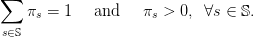
We also adopt new notations. We suppose that the demand W can take a ﬁnite number S of possible values D_s, where s denotes a scenario in the ﬁnite set 𝕊 (S=card(𝕊)). We denote π_s the probability of scenario s ∈ 𝕊, with

∑ πs = 1 and πs > 0, ∀s ∈ 𝕊. s∈𝕊

(4)

Notice that we do not consider scenarios with zero probability.

We consider the stochastic optimization problem

min♯ J(u) = 𝔼 ℙ[j(u, W )]. u∈[0,u ]

(5)

We now show how to rewrite this problem as a linear program. First, we write:

Second, we deduce

Third, we conclude

This is a linear program.

Question 4 Suppose that W follows a uniform distribution over {1, 2,…,w^♯}.

a): [2] Write the linear program (8) under the form adapted to the scicoslab macro linpro.
b): [1] Solve (8) with linpro and obtain the solution to the stochastic optimization problem (5).
c): [1] Compare with the optimal solution of Question 1.
d): [2] Increase the number w^♯ of values taken by the demand W. When can you no longer solve numerically? Compare with the result of Question 1.

3 The newsvendor problem with risk (continuous formulation)

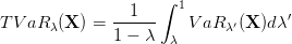
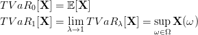
Let λ ∈]0, 1[, that plays the role of a risk level. The Value at Risk of the cost X at level λ ∈]0, 1[ is

V aR λ(X ) = inf{x ∈ ℝ | ℙ (X > x ) < λ}

The Tail Value at Risk of the cost X at level λ ∈]0, 1[ is

∫ 1 T V aR (X) = --1--- V aR ′(X )dλ′ λ 1 − λ λ λ

We have the limit cases:

The Rockafellar-Uryasev formula establishes that

{ + } T VaR λ[X ] = inf 𝔼[(X-−--s)-]+ s , λ ∈ [0, 1[ s∈ℝ 1 − λ

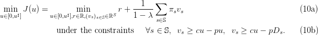
We consider the risk averse stochastic optimization problem

min J (u) = T VaR λ[j(u,W )]. u∈[0,u♯]

(9)

We rewrite this problem as a linear program.

Question 5 Suppose that W follows a uniform distribution over {1, 2,…,w^♯}.

a): [2] Write the linear program (10) under the form adapted to the scicoslab macro linpro.
b): [1] Solve (10) with linpro and obtain the solution to the stochastic optimization problem (9).
c): [1] Compare with the optimal solution of Question 4.

4 The newsvendor problem with backorder (continuous formulation)

Now, we suppose that the newsvendor

pays the unitary purchasing cost c per copy, when he orders stock;
sells a copy at price p; we have that c > p;
can buy extra copies at the unitary backorder cost b, after he observes a demand w larger than the initial order u; we have that b > c
pays the unitary holding cost h for each unsold copy, when the demand w is less than the initial order u.

Therefore, the newsvendor’s costs are

j (u, w) = c ◟u◝◜◞+b [w-− u]+ +h [u-− w-]+ − p◟w◝◜◞ , order ◟ba◝ck◜orde◞r ◟ h◝o◜lding ◞ sold

(11)

where we recall that $x+ = max {x,0}$ .

cc=0.1;pp=10*cc;bb=10*cc;hh=10*cc;

Question 6 We suppose that the demand W follows a uniform distribution over {1, 2,…,w^♯}.

a): [1] Write a row vector criterion made of the values of $J(u) = 𝔼 ℙ[j(u, W )]$ for u ∈{1, 2,…,u^♯}.
b): [1+1] Draw the mapping u ∈ {1, 2,…,u^♯}J(u). Thanks to the scicoslab macro mini (that provides the minimum and the argmin index of a vector), give the numerical value of the decision u^⋆ (optimal order) that minimizes uJ(u).
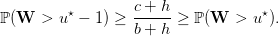
c): [1] Check that, in agreement with the theory, we numerically have that $ℙ(W > u⋆ − 1) ≥ c +-h-≥ ℙ (W > u⋆). b + h$
d): [1+1] For a given value of u, what is the set of values taken by the random variable $j(u, W )$ ? Give a scicoslab formula for the probability distribution of $j(u,W )$ , using probab and decumprobab.
e): [1+1] Draw a histogram of the probability distribution of the random payoﬀ (the opposite of the costs) $− j(u, W )$ for u = u^⋆ (the optimal decision) and for u = 𝔼_ℙ[W] (the naive deterministic solution consisting in ordering the mean demand 𝔼_ℙ[W]). Draw the two histograms on the same picture, so that they have the same scale. Comment on the diﬀerences between the two histograms.
f): [1+1+1] Simulate the trajectory of the cumulated payoﬀs of the newsvendor during one year if, every day, he orders the optimal quantity u = u^⋆. Do the same for u = 𝔼_ℙ[W]. Compare.
g): [4] Multiply the unitary holding cost h by a factor 5. Comment on the changes that you observe.
h): [4] As in Section 2, write the new optimization problem as a linear program. Then, write this latter under the form adapted to the scicoslab macro linpro. Solve with linpro and compare with the optimal solution found above by the direct method.
i): [4] Increase the number w^♯ of values taken by the demand W. When can you no longer solve numerically? Compare with the direct method.