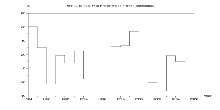
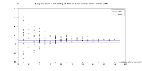
Figure 1: Annual rentability of French stock market (percentage)
1.2 Equivalent annual historical returns
Suppose that you choose an investment duration of T years. You invest at the beginning of any
year between 1988 and 2006 − T + 1, and you compare the final value with what an investment
with safe return would have given on the same duration T. We shall call the return for which both
are equivalent the historical equivalent annual rentability. Letting the year between 1988 and
2006 − T + 1 vary, we obtain, for each investment duration T, an array of historical equivalent
annual rentabilities.
Question 2Compute the historical equivalent annual rentabilities of French stock marketover 1,2, …, 19 consecutive years. Draw a graphic with the number of consecutive years ashorizontal axis and the historical rentabilities as vertical axis.
//
t0=years(1);
tf=years($);
duration=1:(tf-t0+1);
cac40_equi_returns=list();
// cac40_equi_returns(k) is the vector of
// equivalent annual returns over k consecutive years
xset('window',43) ; xbasc() ;
for i=duration;
loc_vec=[];
for j=1:(tf-t0-i+2);
loc=cumprod(1 + 0.01 *cac40_perf_percent(j:(j+i-1)));
loc_vec=[loc_vec,(loc($))^{1/i}-1];
end
plot2d(i*ones(loc_vec),100*loc_vec,style=-1)
cac40_equi_returns(i)=100*loc_vec;
end
xtitle('Long run annual rentability of French stock market from '...
+string(t0) +' to ' +string(tf) ,...
'nb consecutive years','%')
plot2d([0 duration], ones([0 duration]') * [3 8] ); // ,style=[2 3]);
legends([ '3%'; '8%' ] , [1,2], 'ur' );
//
Figure 2: Historical equivalent annual rentabilities (percentage) of French stock market as
function of the duration of investment
1.3 Regular investment
Consider tf− t0 + 1 periods t0, t0 + 1, …, tf (which will be years in this context). Investing a
unitary amount of money at the beginning of period t is supposed to return 1 + ℛ(t) at
the beginning of period t + 1. Thus, if your planning strategy is to invest ℐ(t) at the
beginning of every period t ∈{t0,t0 + 1,…,tf}, you can evaluate your fortune at the horizon
T = tf + 1.
//
function [capital,plus_values]=reg_invest(invest_tab,return_tab)
periods=cumsum(ones(invest_tab)) ;
cumul_invest=cumsum(invest_tab);
// invest_tab : array of regular investment amounts
// return_tab : array of returns
// capital : at last period 1+periods($)
capital=[];
plus_values=[];
for t=periods
capital_loc= ( capital($) + invest_tab(t) ) * (1+return_tab(t)) ;
capital=[capital capital_loc];
plus_values=[plus_values capital_loc-cumul_invest(t) ] ;
end
endfunction
//
Question 3Suppose now that the same strategy is applied with a fixed return ℛ, givingfortune at the horizon T = tf + 1
Which is the fixed rate ℛswhich gives the same final fortune than with a time-varying returnℛ(⋅)?
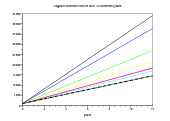
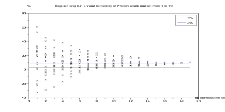
1.4 Equivalent annual historical returns for yearly investment strategy
Question 4Suppose you invest a unitary amount of money at the beginning of every yearin the stock market. Evaluate the equivalent fixed rates, on different horizons, of the strategyconsisting of investing the same amount every year on the stock market.
//
t0=years(1);
tf=years($);
duration=1:(tf-t0+1);
cac40_equi_yearly_returns=list();
// cac40_equi_returns(i) is the vector of
// equivalent annual returns for regular annual investment
// over i consecutive years
xset('window',63) ; xbasc() ;
for i=duration;
loc_vec=[];
for j=1:(tf-t0-i+2);
// loop when the investment horizon i is fixed
return_tab=0.01*cac40_perf_percent(j:(j+i-1));
invest_tab=ones(return_tab);
// unitary amount of regular annual investment
[capital,plus_values]=reg_invest(invest_tab,return_tab);
nb_periods=sum(ones(invest_tab));
fortune=capital($);
retour=equi_return(nb_periods,fortune);
loc_vec=[loc_vec,retour];
end
plot2d(i*ones(loc_vec),100*loc_vec,style=-2);
cac40_equi_yearly_returns(i)=100*loc_vec;
end
xtitle('Yearly investment in French stock market from '...
+string(t0) +' to ' +string(tf) ...
+': annual rentability',...
'nb consecutive years','%')
plot2d([0 duration], ones([0 duration]') * [3 8] );
legends([ '3%'; '8%' ] , [1,2], 'ur' );
//
Figure 3: Historical equivalent annual rentabilities (percentage) of French stock market as
function of the duration of investment in case of yearly investment
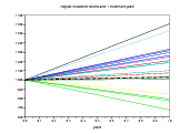
2 Perception of the risk of stock market on different investment durations
2.1 Historical returns on fixed investment duration
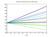
Suppose that you choose an investment duration of T years and an initial capital of 1 000 euros.
Consider that the investment may have started at the beginning of any year between 1988 and
2006 − T + 1. Letting the year between 1988 and 2006 − T + 1 vary, we obtain, for
each investment duration T, an array of historical returns. For T = 1 year, we obtain
2006 − 1988 + 1 = 19 historical returns; for T = 2 years, 18 years; …; for T = 19, only 1 historical
return.
Question 5Draw graphics for T = 1, T = 2, T = 10 with years between 0 and T in abcisseand a straight line joining 1 000 euros to the different historical returns. The straight linesignore the variability during the investment period to focus only on the final return.
//
t0=years(1);
tf=years($);
duration=1:(tf-t0+1);
cac40_hist_returns=list();
// cac40_hist_returns(i) is the vector of
// returns over i consecutive years for 1000 euros investment
for i=duration;
loc_vec=[];
for j=1:(tf-t0-i+2);
loc=1000*cumprod(1 + 0.01 *cac40_perf_percent(j:(j+i-1)));
// for 1000 euros investment
loc_vec=[loc_vec,loc($)];
end
cac40_hist_returns(i)=loc_vec;
end
for i=[1 2 5 8 12]
xset('window',70+i) ; xbasc() ;
plot2d([0 i],[1000*ones(cac40_hist_returns(i)')...
cac40_hist_returns(i)' ]')
xtitle('Stock market historical returns after ' +string(i) +...
' investment years','years')
xpoly([0 i],[1000 1000*(1+.03)^i] ,"lines",0)
p=get("hdl"); //get handle on current entity (here the polyline entity)
p.thickness=6;
p.line_style=5;
end
//
(a) 1 year
(b) 2 years
(c) 8 years
(d) 12 years
Figure 4: French stock market historical returns for same initial investment under different
sequences of consecutive years
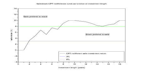
2.2 CPT evaluation of risky historical returns on fixed investment durations
For each number T of consecutive years, one has an array of historical returns, supposed to be the
values taken by a prospect X(T) with equal probabilities. We shall evaluate X(T) with the so
called Cumulative prospect theory or CPT (see [KT79, TK92]), presented in Risk and
Decision.
Question 6Draw the evaluation of the prospect X(T) as a function of investment durationT. Where do you see that the stock market is not chosen if its returns are only perceivedon an annual basis? What is the investment time needed to prefer stock market to a safeinvestment between 2% and 3% [BT95]?
Figure 5: CPT indifference curve between safe or historical stock market rentability as
function of investment length. For instance, a CPT investor is indifferent between investing
5 years in stock markets or 5 years at 6% safe return; a CPT investor prefers investing
10 years in stock markets than 10 years at 9% safe return.
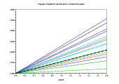
3 Perception of the risk of regular investment in stock market
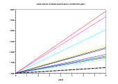
3.1 Historical returns for regular investment in stock market
Suppose that you choose an investment duration of T years and a regular investment of
1 000 euros at the beginning of each year. Consider that the investment may have started at the
beginning of any year between 1988 and 2006 − T + 1. Letting the year between 1988 and
2006 − T + 1 vary, we obtain, for each investment duration T, an array of historical returns. For
T = 1 year, we obtain 2006 − 1988 + 1 = 19 historical returns; for T = 2 years, 18 years; …; for
T = 19, only 1 historical return.
Question 7Draw graphics for T = 1, T = 2, T = 10 with years between 0 and T in abcisseand a straight line joining 1 000 euros to the different historical returns. The straight linesignore the variability during the investment period to focus only on the final return.
//
t0=years(1);
tf=years($);
duration=1:(tf-t0+1);
cac40_yearly_invest_returns=list();
// cac40_yearly_invest_returns(i) is the vector of
// returns for regular annual investment
// over i consecutive years
for i=duration;
loc_vec=[];
for j=1:(tf-t0-i+2);
// loop when the investment horizon i is fixed
return_tab=0.01*cac40_perf_percent(j:(j+i-1));
invest_tab=ones(return_tab);
// unitary amount of regular annual investment
[capital,plus_values]=reg_invest(invest_tab,return_tab);
loc_vec=[loc_vec,capital($)];
end
cac40_yearly_invest_returns(i)=1000*loc_vec;
// for 1000 euros annual investment
end
for i=[1 2 5 8 12]
xset('window',90+i) ; xbasc() ;
plot2d([0 i],[1000*ones(cac40_yearly_invest_returns(i)') ...
cac40_yearly_invest_returns(i)' ]')
xtitle('Regular investment returns after ' +string(i) +...
' investment years','years')
return_tab=0.03*ones(1:i);
// investment of length i
invest_tab=ones(return_tab);
// unitary amount of regular annual investment
[capital,plus_values]=reg_invest(invest_tab,return_tab);
xpoly([0 i],[1000 1000*capital($)] ,"lines",0)
p=get("hdl"); //get handle on current entity (here the polyline entity)
p.thickness=6;
p.line_style=5;
end
//
(a) 1 year
(b) 2 years
(c) 8 years
(d) 12 years
Figure 6: French stock market historical returns for same initial investment under different
sequences of consecutive years
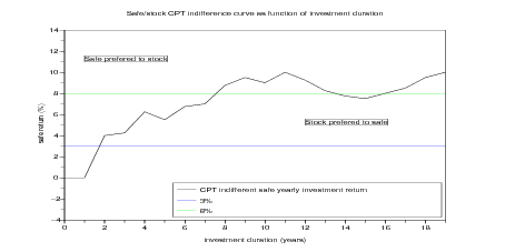
3.2 CPT evaluation of historical returns for regular investment in stock market
Suppose that you choose an investment duration of T years and a regular investment of
1 000 euros at the beginning of each year. For each number T of consecutive years, one has an
array of historical returns, supposed to be the values taken by a prospect Y (T) with equal
probabilities. We shall evaluate X(T) with the CPT.
Question 8Draw the evaluation of the prospect Y (T) as a function of investment durationT. Where do you see that the stock market is not chosen if its returns are only perceivedon an annual basis? What is the investment time needed to prefer stock market to a safeinvestment between 2% and 3% [BT95]?
Figure 7: CPT indifference curve between safe or historical stock market rentability as
function of investment length for yearly investment strategy. For instance, a CPT yearly
investor is indifferent between investing 4 years in stock markets or 4 years at 5% safe return;
a CPT investor prefers investing 10 years in stock markets than 10 years at 8% safe return.
[BT95] Shlomo Benartzi and Richard H Thaler. Myopic loss aversion and the equity
premium puzzle. The Quarterly Journal of Economics, 110(1):73–92, February
1995. available at http://ideas.repec.org/a/tpr/qjecon/v110y1995i1p73-92.html.
[KT79] D. Kahneman and A. Tversky. Prospect theory: an analysis of decision under
risk. Econometrica, 47:263–291, 1979.
[TK92] Amos Tversky
and Daniel Kahneman. Advances in prospect theory: Cumulative representation of
uncertainty. Journal of Risk and Uncertainty, 5(4):297–323, October 1992. available
at http://ideas.repec.org/a/kap/jrisku/v5y1992i4p297-323.html.