Sustainable Management of Fish Stock Based on Spawning Stock Biomass Indicator

Michel De Lara
(last modiﬁcation date: October 10, 2017)

Version pdf de ce document
Version sans bandeaux

1 A single species age-classiﬁed model of ﬁshing
2 ICES precautionary approach and viability
3 Testing the precautionary approach management strategy

1 A single species age-classiﬁed model of ﬁshing

We describe the dynamics of the exploited resource by a controlled dynamic system in discrete time, where the time step is one year. At each time t ∈ ℕ, let us consider N_a(t) the abundance of the stock at age a ∈{1,…,A} and λ(t) the ﬁshing mortality multiplier (control), supposed to be taken at the beginning of period [t,t + 1[. Introducing the state vector N(t) = (N₁(t),…,N_a(t)) (in short: stock), belonging to the state space ℝ₊^A (ℝ₊ the set of nonnegative real numbers), the following dynamic system is considered

N (t + 1) = g(N (t),λ (t)), t = 0,1, 2..., N (0 ) given,

(1)

where the vector function g = (ga) _a=1,…,A is deﬁned for any N ∈ ℝ₊^A and λ ∈ ℝ₊ by

( || g1(N, λ) = φ(SSB (N )), |{ ga(N, λ) = e−(Ma−1+λFa−1)Na− 1, a = 2,...,A − 1 ||| ( gA(N, λ) = e−(MA−1+ λFA −1)NA −1 + π × e− (MA+ λFA)NA.

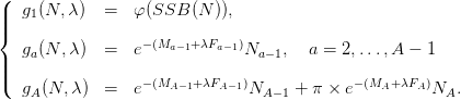(2)

The function φ describes a stock recruitment (S-R) relationship. The spawning stock biomass SSB is deﬁned by

∑A SSB (N ) = γ w N , a a a a=1

(3)

with γ_a the proportion of mature individuals at age and w_a the weight at age. The parameter π ∈{0, 1} is related to the existence of a plus-group to describe the population dynamics for ages greater than A. If we neglect the survivors after age A then π = 0, else π = 1 and the last age class is a plus group.

Here is the data for the Bay of Biscay anchovy. Write the following lines in a ﬁle viab_fish.sce.

  // exec viab_fish.sce
  ////////////////////////////////////////////////////////////////
  // BAY OF BISCAY ANCHOVY
  ////////////////////////////////////////////////////////////////

  ////////////////////////////////////////////////////////////////
  // DATA
  ////////////////////////////////////////////////////////////////

  // parameters for the dynamical model
  sex_ratio=0.5;
  mature=sex_ratio*[1,1,1];// proportion of matures at ages
  weight=10^(-3)*[16,28,36];// mean weights at ages (kg)
  mortality=[1.2,1.2,1.2];// natural mortality
  F=[0.4,0.4,0.4];// exploitation pattern
  pi=1;// plus-group
  A=sum(ones(F));// maximum age

  // SPAWNING STOCK BIOMASS
  function y=SSB(N)
    // spawning stock biomass
    y=(mature .*weight)*N;
  endfunction

  // STOCK-RECRUITMENT RELATIONSHIPS
  // // constant stock-recruitment

  RR=10^6*[14016,7109,3964,696];
  // R_mean R_gm R_min 2002 (ICES) R_min 2004 (ICES)

  function y=R_mean(x)
    y=RR(1);
  endfunction

  function y=R_gm(x)
    y=RR(2);
  endfunction

  function y=R_2004(x)
    y=RR(4);
  endfunction

  // // Ricker stock-recruitment

  a=0.79*10^6;b=1.8*10^(-5);// Ricker coefficients for ton units

  function y=Ricker(x)
    xx=10^{-3}*x;// xx measured in tons
    y=a*(xx .*exp(-b*xx));
  endfunction

  // // Linear stock-recruitment

  r=(500*10^3)*21*0.5*10^{-5};
  function y=linear(x)
    y=r*x;
  endfunction

  // stock_recruitment_list
  SRL=list();
  SRL(1)=list(R_2004,"R_2004");
  SRL(2)=list(R_gm,"R_gm");
  SRL(3)=list(R_mean,"R_mean");
  SRL(4)=list(Ricker,"Ricker");
  SRL(5)=list(linear,"linear");

  // INITIAL VALUES
  N1999=10^6*[4195,2079,217]';
  N2000=10^6*[7035,1033,381]';
  N2001=10^6*[6575,1632,163]';
  N2002=10^6*[1406,1535,262]';
  N2003=10^6*[1192,333,255]';
  N2004=10^6*[2590,254,43]';

  abund_1999_2004=[N1999,N2000,N2001,N2002,N2003,N2004];

  years=1999:2004;
  T=prod(size(years))-1;

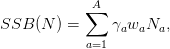
Question 1 Draw trajectories for diﬀerent stock-recruitment relationships with same initial condition and ﬁshing mortality multiplier equal to 1.

Write the following lines in a ﬁle viab_fish.sci.

  // DYNAMICS

  function Ndot=dynamics(N,lambda)
    // depends on the stock-recruitment relationship phi
    // which must be specified before
    mat=diag(exp(-mortality(1:($-1))-lambda*F(1:($-1))),-1)+ ...
        diag([zeros(F(1:($-1))),pi*exp(-mortality($)-lambda*F($))]);
    // sub diagonal terms // diagonal terms
    Ndot=mat*N+[phi(SSB(N));zeros(N(2:$))];
  endfunction

Add the following lines in the ﬁle viab_fish.sce, then execute this latter.

  ////////////////////////////////////////////////////////////////
  // TRAJECTORIES SIMULATION
  ////////////////////////////////////////////////////////////////

  multiplier=1;

  SSBL=list();// spawning stock biomass list

  for i=1:5 do
    phi=SRL(i)(1);// selecting a stock-recruitment relationship
    getf('viab_fish.sci');// coding the dynamics
    //
    traj=[N1999]
    for t=0:(T-1) do
      traj=[traj,dynamics(traj(:,$),multiplier)];
    end
    //
    SSBL(i)=SSB(traj);
    //
  end

  xset("window",0+1);xbasc(0+1);
  plot2d2(years,[SSBL(1)',SSBL(2)',SSBL(3)',SSBL(4)',SSBL(5)',SSB(abund_1999_2004)'])
  xtitle('Anchovy SSB driven by stationary multiplier '+string(multiplier),'time (years)', ...
         'biomass (kg)')
  legends([string(SRL(1)(2));string(SRL(2)(2));string(SRL(3)(2));string(SRL(4)(2));
           string(SRL(5)(2));"historical"],[1,2,3,4,5,6],'ur')

2 ICES precautionary approach and viability

Indicators and reference points

Two indicators are used in the precautionary approach, with associated limit reference points. The ﬁrst indicator, denoted by SSB in (3), is the spawning stock biomass, to which we associate the reference point B_lim > 0. For management advice an additional precautionary reference point Bpa > B_lim is used, intended to incorporate uncertainty about stock state.

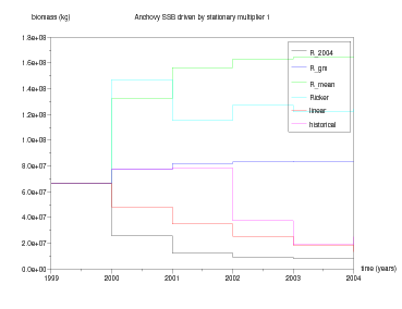
The second indicator, denoted by F, is the mean ﬁshing mortality over a pre-determined age range from a_r to A_r, that is

λ a=∑Ar F(λ ) := A-−--a-+-1- Fa. r r a=ar

(4)

Associated limit reference point is Flim and a precautionary approach reference point Fpa > 0. Acceptable controls λ, according to this reference point, are those for which F(λ) ≤ Flim, as higher F rates might drive SSB below its limit reference point.

Acceptable conﬁgurations

To deﬁne sustainability, we now assume that the decision maker can describe “acceptable conﬁgurations of the system”, that is acceptable couples (N,λ) of states and controls, which form a set 𝔻 ⊂ ℝ₊^A × ℝ₊, the acceptable set. In practice, the set 𝔻 may capture ecological, economic and/or sociological requirements.

Considering sustainable management within the precautionary approach, involving SSB and F indicators, we introduce the following precautionary approach conﬁguration set

𝔻lim := {(N, λ) ∈ ℝA × ℝ+ | SSB (N ) ≥ Blim and F(λ) ≤ Flim}. +

(5)

Viability domains and viable controls

A subset 𝕍 ⊂ ℝ₊^A of the state space ℝ₊^A is said to be a viability domain for dynamics g in the acceptable set 𝔻 if

∀N ∈ 𝕍, ∃ λ ∈ ℝ+, (N, λ) ∈ 𝔻 and g(N,λ ) ∈ 𝕍.

(6)

In other words, if one starts from a stock in 𝕍, there exists an appropriate ﬁshing mortality multiplier such that the system is in an acceptable conﬁguration and the next time step state is also in 𝕍. For example, acceptable equilibria ((N,λ) ∈ 𝔻 and g(N,λ) = N) are viability domains.

Given a viability domain 𝕍, the viable controls associated with any state N ∈ 𝕍 are those controls which let state within the viability domain at next time step, that is which belong to the following (non empty) set

λ𝕍 (N ) := {λ ∈ ℝ+ | (N, λ) ∈ 𝔻 and g(N, λ) ∈ 𝕍}.

(7)

Interpreting precautionary approach in the light of viability

Let us deﬁne the precautionary approach state set

𝕍lim := {N ∈ ℝA | SSB (N ) ≥ Blim}. +

(8)

We shall say that the precautionary approach is sustainable if the precautionary approach state set 𝕍_lim given by (8) is a viability domain for dynamics g in the acceptable set 𝔻_lim.

In [1], we prove the following result.

Result 1 If we suppose that the natural mortality is independent of age, that is M_a = M, and that the proportion γ_a of mature individuals and the weight w_a at age are increasing with age a, the precautionary approach is sustainable if and only if

[ ] inf πe −M x + γ1w1 φ(x) ≥ Blim. x∈[Blim,+∞ [

(9)

that is, if and only if the lowest possible sum of survivors (weighted by growth and maturation) and newly recruited spawning biomass is above Blim.

A constant recruitment is generally used for ﬁshing advice, so the following simpliﬁed condition can be used.

Result 2 Assuming a constant recruitment R, the precautionary approach is sustainable if and only if we have πe^−MB lim + γ₁w₁R ≥ Blim, that is if and only if

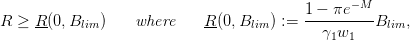− M R ≥ R-(0,Blim) where R-(0,Blim) := 1-−-πe----Blim, γ1w1

(10)

making thus of R(0,Blim) a minimum recruitment required to preserve Blim.

Question 2 Compute R(0,Blim). Compare with the diﬀerent constant recruitment values. Comment.

3 Testing the precautionary approach management strategy

The precautionary approach can be sketched as follows: an estimate of the stock vector N is made; the condition SSB(N) ≥ Blim is checked; if valid, the following usual advice is given

λUA (N ) = max {λ ∈ ℝ+ | SSB (g(N, λ)) ≥ Blim and F (λ) ≤ Flim}.

(11)

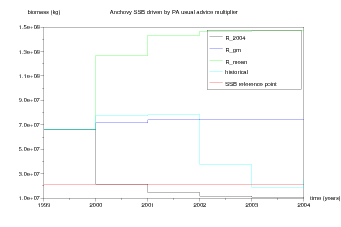
Question 3 Starting from 1999, simulate the eﬀect of the usual advice strategy λ_UA in (11) on dynamics diﬀering by their constant recruitment. Comment the trajectories.

  ////////////////////////////////////////////////////////////////
  //  PRECAUTIONARY APPROACH (PA)
  ////////////////////////////////////////////////////////////////

  // ICES values
  B_lim=21000*10^3;// kg

  // SUSTAINABILITY TEST
  B_ref=B_lim;

  // Constant stock-recruitment case
  M=mean(mortality);
  underlineR=(1-pi*exp(-M))*B_ref/(mature(1)*weight(1))

  for i=1:3 do
    loc_list=SRL(i);loc_func=loc_list(1);
    // local variables necessary with old versions of Scilab
    if loc_func(0) > underlineR then
      //  if  SRL(i)(1)(0) > underlineR then
      printf('\n Precautionary approach sustainable with constant recruitment '+ ...
             string(SRL(i)(2)));
    else
      printf('\n Precautionary approach NOT sustainable with constant recruitment '+ ...
             string(SRL(i)(2)));
    end
  end

  // FEEDBACK
  delta=0.1,// control precision

  function u=max_UA(N,lambda_max,B)
    // usual PA advice
    lambda=0;
    check=1;
    while check==1 & lambda <= lambda_max do
      NN=dynamics(N,lambda);
      check=sign(SSB(NN)-B);
      lambda=lambda+delta;
    end
    u=lambda-delta-delta;
  endfunction

  // TRAJECTORIES
  function [ssb_traj,lambda_traj]=trajectory(N,horizon,feedback)
    // returns SSB and multiplier under strategy "feedback"
    s_traj=N;
    ssb_traj=SSB(N);
    lambda=feedback(N);
    c_traj=lambda;
    for t=0:(horizon-1) do
      NN=dynamics(s_traj(:,$),c_traj($));
      lambda=feedback(NN);
      c_traj=[c_traj,lambda];
      s_traj=[s_traj,NN];
      ssb_traj=[ssb_traj,SSB(NN)];
    end
    lambda_traj=c_traj
  endfunction

  // SIMULATIONS
  N0=N1999;
  B_viable=B_ref;
  lambda_max=2;

  function u=feedback_UA(N)
    u=max_UA(N,lambda_max,B_viable)
  endfunction

  SSBUAL=list();// spawning stock biomass, with PA usual advice, list

  for i=1:3 do
    phi=SRL(i)(1);// selecting a stock-recruitment relationship
    getf('viab_fish.sci');// coding the dynamics
    //
    traj=[N1999]
    [ssb_traj,lambda_traj]=trajectory(N0,T,feedback_UA);
    //
    SSBUAL(i)=ssb_traj;
    //
  end

  xset("window",10+1);xbasc(10+1);
  plot2d2(years, ...
          [SSBUAL(1)',SSBUAL(2)',SSBUAL(3)',SSB(abund_1999_2004)',B_viable*ones(years)'])
  xtitle('Anchovy SSB driven by PA usual advice multiplier','time (years)','biomass (kg)')
  legends([string(SRL(1)(2));string(SRL(2)(2));string(SRL(3)(2));"historical";
           'SSB reference point'],[1,2,3,4,5],'ur')

Question 4 Propose the largest Blim such that the precautionary approach is sustainable with every observed constant recrutment. Illustrate the result with simulations.

References

[1] M. De Lara, L. Doyen, T. Guilbaud, and M.J. Rochet. Is a management framework based on spawning stock biomass indicator sustainable? a viability approach. ices Journal of Marine Science, 2006. In press.

Formations

Départements

Pratique

Recherche

Management of Energy

Management of Renewable Resources and Biodiversity

Management of Exhaustible Resources

Models in Life Science

Miscellaneous