


| L'École des Ponts ParisTech est membre fondateur de |
L'École des Ponts ParisTech est certifiée |


|
|


We consider a dam manager intenting to maximize the intertemporal payoff obtained by selling power produced by water releases, when the water inflows (rain, outflows from upper dams) are random. However, the manager must also respect a minimal volume during the Summer months for tourism reasons.
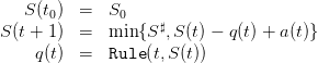
We model the dynamics of the water volume in a dam by
 |
with
 , made of water volumes, where
  is the maximum
dam volume,
is the maximum
dam volume,
 , where q♯ is the maximum which can be turbined by time unit
(and produce electricity),
, where q♯ is the maximum which can be turbined by time unit
(and produce electricity),
![s(t) = [S (t) − q(t) + a(t) − S ♯]
+](dam_viability5x.png) the spilled volume
the spilled volumeThe dam manager is supposed to make a decision, here turbining q(t) at time t, before knowing the water input a(t). Such a case is called decision-hazard. The constraint on the water turbine q(t) is
 | (1) |
A scenario is a sequence of uncertainties:
 | (2) |
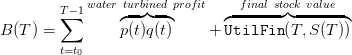
The manager original problem is one of payoff maximization where turbining one unit of water has unitary price p(t). On the period from t0 to T, the payoffs sum up to
 | (3) |
where
 | (4) |
of prices is supposed to be known in advance (in other models, it could be progressively revealed to the manager),
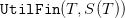 gives value to the water volume in the dam at the horizon
T.
gives value to the water volume in the dam at the horizon
T.
For “tourism” reasons, the following constraint is imposed

In what follows, we shall be more specific about the sense with which this constraint has to be satisfied, namely in probability.
A strategy Rule : 𝕋 × 𝕏 → 𝕌 assigns a water turbined 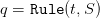 to any state S of dam stock
volume and to any decision period t ∈ 𝕋. Once given, we obtain uncertain volume trajectories
to any state S of dam stock
volume and to any decision period t ∈ 𝕋. Once given, we obtain uncertain volume trajectories
 and turbined trajectories
  produced by the “closed-loop” dynamics
 | (5) |
and function of the scenario a(⋅). Thus, in the end, we obtain an uncertain payoff
 | (6) |
where  and
and  are given by (5).
We suppose that sequences of uncertainties  are random variables with a
known probability distribution ℙ on the set
are random variables with a
known probability distribution ℙ on the set  .
.
We suppose that the random variables  are independent with
distribution
are independent with
distribution  on the set
  :
:
 | (7) |
Notice that the random variables  are independent, but that they are not
necessarily identically distributed. This allows us to account for seasonal effects (more rain in
autumn and winter).
are independent, but that they are not
necessarily identically distributed. This allows us to account for seasonal effects (more rain in
autumn and winter).
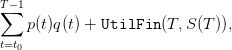
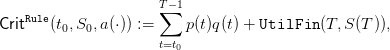
To each strategy Rule, we associate the expected payoff
![∑T−1
𝔼 [CritRule(t0,S0,a(⋅))] = 𝔼[ p(t)q(t) + UtilFin (T, S(T ))],
t=t0](dam_viability26x.png) | (8) |
where the expectation 𝔼 is taken with respect to the probability ℙ.
The dynamic programming equation associated with the problem of maximizing the expected payoff (8)
![T∑− 1
max 𝔼[ p(t)q(t) + UtilFin (T, S(T ))]
t=t0](dam_viability27x.png) | (9) |
is
![final payoff
◜-------◞◟------◝
V (T,S ) = UtilFin (T, S(T )),
♯
V(t,S ) = max ♯ 𝔼a(t)[ p◟(◝t)◜q◞ +V (t + 1,m◟in-{S-,S-−◝◜-q +-a-(t)}◞ )],
q∈{0,1,2,...,min{S,q }} instant. payoff future stock volume](dam_viability28x.png) | (10) |
where the expectation 𝔼 is taken with respect to the probability in (7).
We know will make numerical simulations, and try different strategies. We shall consider a daily management over one year
 | (11) |
with
 | (12) |
where we say that, during one week, one can turbine at maximum 40% of the dam volume, and that during one week of full water inflows, an empty dam can be half-filled.
The sequence of prices is known in advance. We shall produce it by one sample from the expression
 | (13) |
where  is drawn from a sequence of i.i.d. uniform random variables in
 ![[− 1∕2,1 ∕2]](dam_viability33x.png) .
.
The probability of water inflows (from zero to the maximum  ) is known in
advance.1
) is known in
advance.1
Copy the following Scilab code into a file DamData.sce.
Copy the following Scilab macros into the same file DamData.sce.
In the macro trajectories, the output CC is the mean payoff averaged over the scenarios: by the law of large numbers, CC is an approximation of the expected payoff if the number of scenarios is large enough (Monte Carlo method).
Copy the following Scilab code into the file Damoptimality.sce.
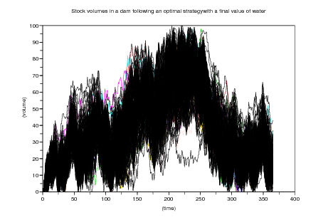
We first consider that the final “value of water” is zero:
 | (14) |
Question 1 Picture the trajectories of the stocks corresponding to the optimal strategy.
Evaluate the optimal expected payoff, and compare it with the value function  evaluated at the initial time t0 and the initial stock
  . Explain why these two quantities
should be close. What do you observe for the final stocks? Explain why.
. Explain why these two quantities
should be close. What do you observe for the final stocks? Explain why.
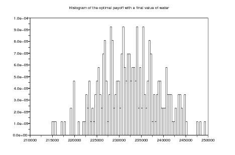
Till now, there was no gain in leaving water in the dam at the ultimate decision period. From now
on, we consider that the “value of water”  is given by
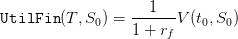 | (15) |
where  is a discount factor. We shall take
  when
when  days.
days.
Copy the following Scilab code into the file DamOptimality.sce.
Question 2 Picture the trajectories of the stocks corresponding to the optimal strategy.
Evaluate the optimal expected payoffs for different values of the initial stock  , and
compare them with the value function
, and
compare them with the value function  evaluated at the initial time t0 and the
initial stock
evaluated at the initial time t0 and the
initial stock  . Display the histogram of the optimal payoff. Compare the mean of the
optimal payoff with the upper and lower bounds of the distribution.
. Display the histogram of the optimal payoff. Compare the mean of the
optimal payoff with the upper and lower bounds of the distribution.
Let  denote an optimal stock trajectory.
The payoff at time t ∈ 𝕋 is
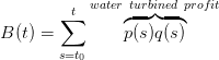
and
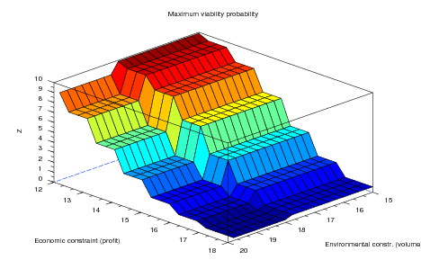
We propose an alternative stochastic viability formulation to (9)-(16) under the form
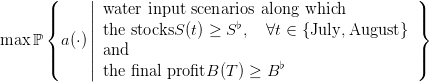 | (17) |
The dynamic programming equation associated with the problem of maximizing the viability probability (17) is
![final constraint
◜--◞◟-◝
V (T,S,B ) = 1{B≥B ♭} ,
V (T − 1,S,B ) = max 𝔼a (T− 1)[1 ♭
q∈ {0,1,2,...,min{S,q♯}} {S≥S ,T−1∈{July,August}
×V (t + 1,min {S♯,S − q + a(T − 1)},
B + p(T − 1)q + UtilFin (T,min {S♯,S − q + a(T − 1)})],
instantaneous constraint
◜--------◞◟---------◝
V(t,S,B ) = max ♯ 𝔼a (t)[1{S(t)≥S♭,t∈{July,August}}
q∈ {0,1,2,...,min{S,q}}♯
×V (t + 1,m◟in-{S-,S(t) −◝◜-q(t) +-a(t)}◞, B◟-+◝p◜(t)q◞ )], ∀t = t0,...,T − 2,
future stock volume future payoff](dam_viability57x.png) | (18) |
where the expectation 𝔼 is taken with respect to the probability (7). Notice that the equation for
t = T − 1 takes into account the term  in the payoff.
Copy the following Scilab code into the file DamViability.sce.
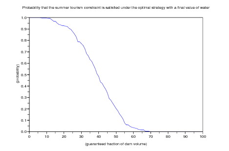
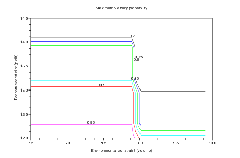
Question 4 Compute the maximal viability probability. Deduce the viability kernels with confidence levels 100%, 95% and 90%.
Copy the following Scilab code into the file DamViability.sce.
Question 5 Launch the above code (maybe you will have to reduce the time step, or the horizon, and adapt the code in consequence if the computation takes too much time). Visualize the maximal viability probability starting from an almost full dam. Draw iso-probability curves. Comment on what you observe.
D. P. Bertsekas. Dynamic Programming and Optimal Control. Athena Scientific, Belmont, Massachusets, second edition, 2000. Volumes 1 and 2.
M. De Lara and L. Doyen. Sustainable Management of Natural Resources. Mathematical Models and Methods. Springer-Verlag, Berlin, 2008.
| L'École des Ponts ParisTech est membre fondateur de |
L'École des Ponts ParisTech est certifiée |
|
|
|


