Contents

1 A two-dimensional open pit mine optimal extraction model

Open pit mines are generally designed with the help of so-called block models, or resource models. These latter represent the material inside the pit using millions of blocks with given shape. Open pit mines extraction is submitted to physical restrictions: only blocks at the surface may be extracted; a block cannot be extracted if the slope made with one of its neighbors is too high, due to geotechnical constraints on mine wall slopes.

In essence, exploiting an open pit mine can be seen as selecting an admissible extraction sequence of blocks where, by admissible, we mean that the above physical restrictions are satisfied. Among all admissible extraction sequences, of particular economic interest are those which are the more profitable.

Block model

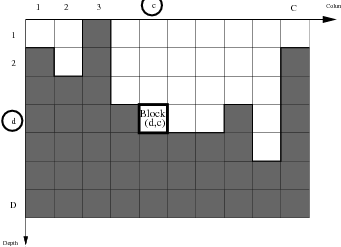
For simplicity, we shall consider a two-dimensional mine [1] as in Fig. 1. Each block is a two-dimensional rectangle identified by its vertical position d ∈{1,…,D} (d for depth) and by its horizontal position c ∈{1,…,C} (c for column).

---

---

Dynamics

We assume that blocks are extracted sequentially under the following hypothesis [2, 1]:

• it takes one time unit to extract one block;
• only blocks at the surface may be extracted;
• a block cannot be extracted if the slope made with one of its two neighbors is too high, due to geotechnical constraints on mine wall slopes (the rule is mathematically decribed in the sequel);
• a retirement option is available where no block is extracted.

States and admissible states

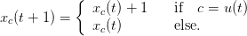
Denote discrete time by t = 0, 1,…,T, where an upper bound for the number of extraction steps is the number C × D of blocks (it is in fact strictly lower due to slope constraints). At time t, the state of the mine is a profile

where x_c(t) ∈{1,…,D + 1} is the vertical position of the top block with horizontal position c ∈{1,…,C} (see Fig. 1). The initial profile is x(0) = (1, 1,…, 1) while the mine is totally exhausted in state x = (D + 1,D + 1,…,D + 1).

An admissible profile is one that respects local angular constraints at each point, due to physical requirements. A state x = (x₁,…,x_C) is said to be admissible if the geotechnical slope constraints are respected in the sense that

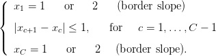(1)

Denote by 𝔸 ⊂{1,…,D + 1}^C the set of admissible states satisfying the above slope constraints (1).

Controlled dynamics

A decision is the selection of a column in ℂ = {1,…,C}, the top block of which will be extracted. A decision may also be the retirement option, that we shall identify with an additional fictituous column denoted ∞. Thus, a decision u is an element of the set ℂ = ℂ ∪{∞} = {1,…,C,∞}.

At time t, if a column u(t) ∈{1,…,C} is chosen at the surface of the open pit mine, the corresponding block is extracted and the profile x(t) = x₁(t),…,x_C(t) becomes

In case of retirement option u(t) = ∞, then x(t + 1) = x(t) and the profile does not change. In other words, the dynamics is given by x(t + 1) = DYN(x,u) where

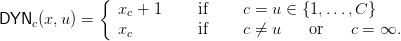(2)

Indeed, the top block of column c is no longer at depth x_c(t) but at x_c(t) + 1, while all other top blocks remain.

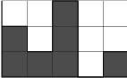
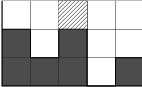
Starting from state x = (2, 3, 1, 4, 3) in Figure 2 and applying control u = 3, one obtains the following state (2, 3, 2, 4, 3) as in Figure 3.

---

---

---

---

Decision constraints

Not all decisions u(t) = c are possible either because there are no blocks left in column c (x_c = D + 1) or because of slope constraints.

When in state x ∈ 𝔸, the decision u ∈ℂ is admissible if the future profile DYN(x,u) ∈ 𝔸, namely if it satisfies the geotechnical slope constraints. This may easily be transformed into a condition u ∈ 𝔹(x), where

(3)

Intertemporal profit maximization

The open pit mine optimal scheduling problem consists in finding a path of admissible blocks which maximizes an intertemporal discounted extraction profit. It is assumed that the value of blocks differs in depth and column because richness of the mine is not uniform among the zones as well as costs of extraction. The profit model states that each block has an economic value Rent(d,c) ∈ ℝ, supposed to be known.¹ By convention Rent(d,∞) = 0 when the retirement option is selected. Selecting a column u(t) ∈ ℂ at the surface of the open pit mine, and extracting the corresponding block² at depth x_u(t)(t) yields the value Rentx_u(t)(t),u(t). With discount rate rf ≥ 0 and discount factor 0 ≤ ≤ 1, the optimization problem is sup _u(⋅) ∑ _t=0^+∞()^tRentx _u(t)(t),u(t). Notice that the sum is in fact finite, bounded above by the number T − 1 of blocks. Thus, we shall rather consider³

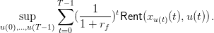(4)

Dynamic programming equation

The maximization problem (4) may theoretically be solved by dynamic programming. The value function 𝒱(t,x) solves 𝒱(T,x) = 0 and

(5)

However, due to numerical considerations (curse of dimensionality), we shall have to introduce a new, and more parcimonious, state before applying the dynamic programming algorithm.

2 Dynamic programming algorithm

Numerical considerations

To give a flavor of the complexity of the problem, notice that 4 columns (C = 4) each consisting of nine blocks (D = 9) give 10 000 states (𝕏^♯ = 10⁴), while this raises to 10^20 000 if we assume that the surface consists of 100 × 100 columns (C = 10 000) with ninety-nine blocks (D = 99) .

However, the set 𝔸 of acceptable states has a cardinal 𝔸^♯ which is generally much smaller than 𝕏^♯. To see this, let us introduce the mapping x = (x ₁,…,x_C)φ(x) = (x₁,x₂ − x₁,…,x_C − x_C−1). Let x ∈ 𝔸 and y = φ(x). Since x satisfies the admissibility condition (1), y necessarily satisfies y₁ ∈{1, 2} and sup _c=2,…,C≤ 1. Hence, card(𝔸) ≤ 2 × 3^C−1 and the dynamic programming algorithm will be released with the new state y = (y₁,…,y_C) ∈{1, 2}×{−1, 0, 1}^C−1 corresponding to the increments of the state x. Table 2 provides some figures.

A new incremental state

The dynamic programming algorithm will be released with the new state

(6)

corresponding to the increments of the state x given by the inverse mapping

(7)

By construction, x = φ⁻¹(y) always satisfies the slope constraints (1). However, it does not always correspond to a mine profile state. Indeed, some y ∈ 𝕐 give x = φ⁻¹(y) ⁄∈ 𝕏 = {1,…,D + 1}^C: for instance y = (1,−1,−1,…,−1) yields x = (1, 0,−1,−2,…,C − 2).

The dynamics (x,u)DYN(x,u) now becomes (y,u)G(y,u) = φDYN(φ⁻¹(y),u):

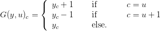(8)

Labelling the states

The new state set 𝕐 is a product space: we shall label its elements with integers. Let Q ∈{−1, 0, 1, 2,…} be the unique integer such that

(9)

Consider the following labelling mapping⁴

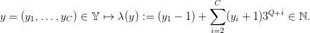(10)

The inverse mapping of λ is given as follows. Any integer z ∈{0, 1,…, 3^Q+C+1} may be decomposed in the basis {1, 3^Q+2,…, 3^Q+C} as

(11)

for i = 2,…,C. Thus (y₁,…,y_C) = λ⁻¹(z) is given by y ₁ = z₁ + 1 ∈{1,…, 3^Q+2} and y_i = z_i − 1 ∈{−1, 0, 1} for i = 2,…,C. Denote by ℤ_a ⊂{0, 1,…, 3^Q+C+1} those z to which corresponds an admissible state x = φ⁻¹λ⁻¹(z) ∈ 𝔸.

The dynamics (8) is translated in

(12)

because of the expression (11) for z.

Let z ∈ ℤ_a. Of course, z′ = H(z,u) corresponds to an admissible state (z′∈ ℤ_a) if and only if u is admissible for the state x = φ⁻¹λ⁻¹(z) ∈ 𝔸, property that we shall denote by u ∈ 𝕌_a(z) ⊂{1,…,C}.

3 Simulating extraction strategies

3.1 Data

Copy the file "marvin_7440_valores.txt" in your local directory. Then, create a file "data.sce" in your local directory containing the following code.

3.2 Upper and lower bounds for the value of the mine

The so called value of the mine is 𝒱(0,x(0)) given by (4).

3.3 Optimal trajectories simulation

State labelling

Copy the following code in a file "mine_DP_label.sce"

Dynamic programming algorithm

Copy the following code in a file "mine_DP_algorithm.sce"

Visualization

Copy the following code in a file "mine_visualize.sce"

Optimal trajectories simulation

Copy the following code in a file "mine_DP_trajectories.sce"

References