
| L'École des Ponts ParisTech est membre fondateur de |
L'École des Ponts ParisTech est certifiée |


|
|


This pratical work will follow the example worked out in M. De Lara’s first lecture. The
computations will be performed using nsp (a Matlab like simulation language). In order to launch
nsp just use the Nsp entry in the menu Applications/Science. You will need a specific nsp toolbox
called qhull to perform Voronoi tesselation. In order to load it, just type within nsp:
exec('COURSES/qhullnsp/loader.sce');
Consider two independent random variables  and
and  , each with a uniform probability
distribution over
, each with a uniform probability
distribution over ![[− 1,1]](voronoi2x.png) (zero mean, variance
(zero mean, variance  ). The unique decision variable
  may
only use the observation of
may
only use the observation of  (which we view as the initial state
  ). The final state
  is equal to
  . The goal is to minimize
  , where
  is a given
“small” positive number (“cheap control”). The statement is thus
is a given
“small” positive number (“cheap control”). The statement is thus
 | (1) |
We have that
 |
 and
and  are centered
independent random variables and since
are centered
independent random variables and since  is measurable with respect to
  . The first two
terms yield twice the variance
. The first two
terms yield twice the variance  of the noises. Therefore, we remain with the problem of
minimizing
of the noises. Therefore, we remain with the problem of
minimizing
 | (2) |
by choosing  as a measurable function of
  . One can see that the solution is given
by
. One can see that the solution is given
by

and the corresponding optimal cost is readily calculated to be
 | (3) |
Question 1 Use the following code to recover previous results by both numerical integration (nsp function intg) and Monte Carlo simulations. Choose and code an other feedback and compare the associated cost with the optimal cost.
We now proceed to some discretization of this problem. To that purpose, we first consider  noise trajectories
  which are
  sample of the two-dimensional vector
 . Those samples will serve to approximate the cost expectation by a usual Monte
Carlo averaging.
. Those samples will serve to approximate the cost expectation by a usual Monte
Carlo averaging.
However, in this process, we must also consider  corresponding realizations
  of the random decision variable
  . But we must keep in mind that this random
variable should be measurable with respect to the first component
. But we must keep in mind that this random
variable should be measurable with respect to the first component  of the previous
vector.
of the previous
vector.
To that purpose, we impose the constraint
 | (4) |
which prevents  from taking different values whenever
  assumes the same value in any
two sample trajectories.
assumes the same value in any
two sample trajectories.
When Constraint (4) is never active, then we have to compute a different control value for each sample and the cost is:
 | (5) |
This expression must be minimized in  for every
  under the constraint (4). This
yields the optimal value
under the constraint (4). This
yields the optimal value
 | (6) |
and the corresponding contribution to the cost  . This is of order
  , and so
is the average over
, and so
is the average over  samples
 | (7) |
even when  goes to infinity. This is far from the actual optimal cost given by (3).
Question 2 Use the function grand to obtain a set of N=2500 samples of (W0,W1).
Assuming that the N values that you obtain for W0 are one by one distinct, compute the
optimal cost of the discrete problem.
Optional question: set N=1000000 and check if all the values for W0 are one by one distinct
(use function unique and type help unique to get the online manual). If not, propose a
modification of the code to handle this case in order to compute the discrete optimal cost.
However, any admissible solution (any  such that
  is measurable w.r.t.
  ) cannot
achieve a cost which is better than the optimal cost (3). The value (7) is just a “fake”
cost estimation. The resolution of the discretized problem derived from the previous
Monte Carlo procedure yielded an optimal value
) cannot
achieve a cost which is better than the optimal cost (3). The value (7) is just a “fake”
cost estimation. The resolution of the discretized problem derived from the previous
Monte Carlo procedure yielded an optimal value  (see (6)) associated with each
sample noise trajectory represented by a point
(see (6)) associated with each
sample noise trajectory represented by a point  in the square
 ![[− 1,1 ]2](voronoi49x.png) . Hence,
before trying to evaluate the cost associated with this “solution”, we must first derive
from it an admissible solution for the original problem, that is, a random variable
. Hence,
before trying to evaluate the cost associated with this “solution”, we must first derive
from it an admissible solution for the original problem, that is, a random variable  over
over ![Ω = [− 1,1]2](voronoi51x.png) , but with constant value along every vertical line of this square
(since the abscissa represents the first component
, but with constant value along every vertical line of this square
(since the abscissa represents the first component  of the 2-dimensional noise
 ).
).
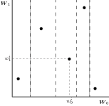
A natural choice is as follows:
 sample points so that the first component
  is increasing
with
is increasing
with  ;
;
 vertical strips by drawing vertical lines in the
middle of segments
vertical strips by drawing vertical lines in the
middle of segments ![[wi0,wi0+1]](voronoi58x.png) , that is, the
, that is, the  -th strip is
 ![[ai−1,ai] × [− 1,1 ]](voronoi60x.png) with
with
 for
for 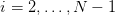 ,
,  , and
, and  ;
;
 as the function of
  which is piecewise constant
over the square divided into those
which is piecewise constant
over the square divided into those  strips, using of course the optimal value
  given
by (6) in strip
given
by (6) in strip  ; that is, we consider
![N
∑ i
U (w ) = u 1[ai−1,ai]×[−1,1](w ),
i=1](voronoi70x.png) | (8) |
where  ranges in the square
 ![[− 1,1]2](voronoi72x.png) and
and  is the function which takes the value 1
in
is the function which takes the value 1
in  and 0 elsewhere.
Since this is an admissible solution for the original (continuous) problem, the corresponding
cost value  can be evaluated. Here, the expectation is over the argument
  considered as a random variable over the square with uniform distribution (the calculation of this
expectation is done analytically).
considered as a random variable over the square with uniform distribution (the calculation of this
expectation is done analytically).
According to (2), this expected cost is easily evaluated as
 | (9) |
Question 3 Compute the optimal cost for the real problem obtained with the feedback (8) for a given sample of (W0,W1). You will have to do the following steps:
Although this is an “expected” cost, it is still a random variable since  and
and  are functions of
the
are functions of
the  ’s which result from random drawings (
 also depends upon the
  ’s). The optimal
cost being itself a random variable, compute by Monte Carlo its mean and standard deviation for
different values of N.
’s). The optimal
cost being itself a random variable, compute by Monte Carlo its mean and standard deviation for
different values of N.
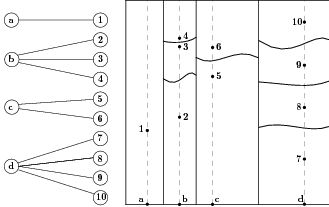 The question is thus: how to
formulate another constraint translating the informational constraint in the discretized problem
more effective than (4)? An obvious answer is that, in our collection of sample trajectories used in
the discrete optimization problem, there should really be distinct samples with the same value of
component
The question is thus: how to
formulate another constraint translating the informational constraint in the discretized problem
more effective than (4)? An obvious answer is that, in our collection of sample trajectories used in
the discrete optimization problem, there should really be distinct samples with the same value of
component  .
.
Admittedly, if the scenarios are produced randomly (according to the joint uniform probability
law of  over the square
 ![[− 1,1] × [− 1,1]](voronoi86x.png) ), or if they have been recorded from real life
observations, there is a probability zero that a tree shape will pop up spontaneously, for any
arbitrary large but finite
), or if they have been recorded from real life
observations, there is a probability zero that a tree shape will pop up spontaneously, for any
arbitrary large but finite  .
.
In the case of our example, since  and
and  are known to be independent (the white
noise case), any element in a set of
are known to be independent (the white
noise case), any element in a set of  samples of
  can be combined with the
same, or
can be combined with the
same, or  distinct, sets of
  samples of
  to produce such a tree. Even
if
to produce such a tree. Even
if  and
and  were not independent, one could first generate
  samples of
 using the marginal probability law of this variable, and then, using each sample
 and the conditional probability law of
  knowing that
  assumes the
value
assumes the
value  , one could generate
  associated samples
  of
of  (“sons” of that
 ).
).
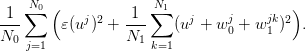
To fix notations, we consider scenarios 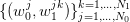 and we introduce the following
additional symbols:
and we introduce the following
additional symbols:
 | (10) |
Notice that  can be interpreted as an estimate of the conditional expectation of
  knowing that
  . Likewise,
  can be interpreted as an estimate of the conditional
second order moment.
can be interpreted as an estimate of the conditional
second order moment.
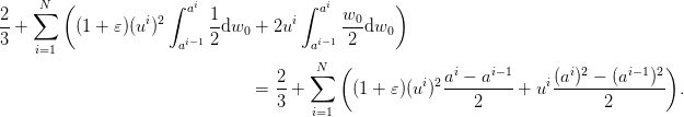
The cost of the discretized problem is
The minimizer is
 | (11) |
to be compared with (6). This yields the optimal cost
 | (12) |
to be compared with (7) and (3). If we assume that the estimates (10) converge towards
their right values (respectively, 0 and 1/3) as  goes to infinity, then (12) gets close
to
goes to infinity, then (12) gets close
to
Now, the expression  can also be viewed as an estimate of the second order
moment of
can also be viewed as an estimate of the second order
moment of  and, if we assume that it converges to the true value 1/3 when
  goes to
infinity, then we recover, in the limit, the true optimal cost (3). Therefore, unlike with the previous
naive Monte Carlo method (see (7)), here the optimal cost obtained in the discrete problem
appears to converge to the right value.
goes to
infinity, then we recover, in the limit, the true optimal cost (3). Therefore, unlike with the previous
naive Monte Carlo method (see (7)), here the optimal cost obtained in the discrete problem
appears to converge to the right value.
As we did earlier (see (9)), it is also interesting to evaluate the real cost associated with an
admissible solution derived from the collection of “optimal” values (11) by plugging those values
into the formula (8) (with  replaced by
  ). Again, we have appealed to a computer
program using 100 experiments, each consisting in:
). Again, we have appealed to a computer
program using 100 experiments, each consisting in:
 values
  at random;
 values
  at random;
 ’s (see (10)), the
  ’s (see (11)) and forming the admissible
solution (8) (
’s (see (11)) and forming the admissible
solution (8) ( replaced by
  ) with those values after reordering the indices
  so that
  is increasing with
  ;
;
 by analytic integration w.r.t. the couple
 with uniform probability distribution over the square
 ![2
[− 1,1]](voronoi136x.png) .
.
Question 4 Compute the optimal cost for the real problem obtained with the feedback (8) for a given tree sample of (W0,W1). The optimal cost being itself a random variable, compute by Monte Carlo its mean and standard deviation for different values of N.
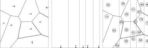
We consider now an alternative approach consisting in independent discretizations of noise and information. The noise is discretized using a voronoi tesselation (Nc cells) and the control is discretized using vertical strips (Ns strips). As shown in the slides, we need to solve Ns optimization problems (one problem for each strip), formulated as follows :

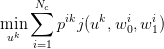 |
 is the probability weight of the intersection of cell
  with strip
 .
.
Question 5
Note that you can use the macro SquareBV in order to compute the surfaces of the intersections of the cells of a voronoi tesselation and of a given rectangle.
| L'École des Ponts ParisTech est membre fondateur de |
L'École des Ponts ParisTech est certifiée |
|
|
|


