Optimal control of a domestic microgrid

SOWG
(last modiﬁcation date: October 10, 2017)

Version pdf de ce document
Version sans bandeaux

1 Problem statement, formalisation and data
2 Simulation and evaluation of given policies
3 Solving by two diﬀerent methods
A Discretization and interpolation schemes

1 Problem statement, formalisation and data
1.1 Problem statement
1.2 System’s dynamic
1.2.1 Battery dynamic
1.2.2 Hot water tank dynamic
1.3 Criterion: operational costs
1.4 Optimization criterion
2 Simulation and evaluation of given policies
2.1 Evaluation of a policy
2.2 Simulation of a given policy
3 Solving by two diﬀerent methods
3.1 Model Predictive Control
3.2 Stochastic Dynamic Programming
3.3 Comparison between diﬀerent policies
A Discretization and interpolation schemes
A.1 Discretization
A.2 Interpolation

Abstract

1 Problem statement, formalisation and data

1.1

1.1 Problem statement

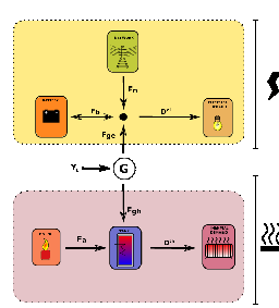
We consider here a house equipped with a thermal hot water tank, a combined heat and power generator (CHP) and a battery. This house has two systems to satisfy its energetical needs: a thermal system for heating, and an electrical system to satisfy its electrical demand. These two systems are coupled together via the CHP, rendering the optimal control diﬃcult to ﬁnd.

The CHP is a generator which produces both electricity and heat while burning gas. The power of the CHP can not be modulated: it produces always the same amount of heat and electricity.

A battery can store the potential surplus of electricity (especially when demand is low), and the house is connected to the grid to import electricy if necessary. The heat produced by the CHP is stored in a hot water tank. Hot water is withdrawn from this tank to satisfy thermal demand.

We aim to decrease the operational costs while taking into account that:

the electrical price depends upon time, as shown in Figure 2,
electrical and thermal demands are highly variable (the evolution of these demands are displayed in Figure 3).

Figure 1: Diﬀerent systems constituting the domestic microgrid.

Figure 2: Electrical price

Figure 3: Diﬀerent scenarios for demand

1.2

1.2 System’s dynamic

We model our system with discrete linear equations, stating the evolution of the system between two timesteps t and t + 1. Controls are computed at the begining of the time interval [t,t + 1[, and are applied all along this interval. That gives a discrete time optimal control problem.

We control here the system during one day, at a 15mn timestep.

1.2.1

1.2.1 Battery dynamic

B_t is the energy stored inside the battery at time t. The battery’s dynamic is the following:

Bt+1 = Bt + ΔtFB,t.

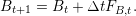(1)

Battery’s constraints The battery’s level must remain greater than a given level otherwise its life expectancy decreases much more quickly. Usually, it is speciﬁed that this level remains between 30% and 90% of the maximum level of charge. The charge and discharge are also bounded by a maximum rampage rate ΔB. These two constraints write:

B ♭ ≤ Bt ≤ B ♯.

(2)

and

− ΔB ≤ Bt+1 − Bt ≤ ΔB

(3)

1.2.2

1.2.2 Hot water tank dynamic

We have two inputs for the hot water tank:

the heat F_gh,t = (1 − α)P_chp,t produced by the CHP,
the heat F_A,t produced by the auxiliary burner,

and one output: the thermal demand of the house D_t^th.

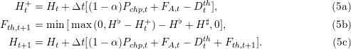
We denote the tank’s level H_t, denoting the energy stored inside the tank at time t (in kWh). This level is bounded:

H ♭ ≤ Ht ≤ H ♯.

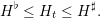(4)

The hot water tank is modelled with:

All these equations are designed so as the constraints 4 are satisﬁed for all demand D_t^th.

The recourse variable F_th,t+1 is penalized afterward in the cost function.

1.3

1.3 Criterion: operational costs

Electrical exchange We denote F_N,t the electricity imported from the grid at time t.

The balance equation between production and demand in the upper electric part in Figure 1.1 writes:

αPchp,t + FN,t = Detl+ FB,t

(6)

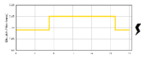
The electricity imported from the network is being paid at a tariﬀ π_t^el, which depends upon time. The price scenario π_{t_i}^el,…,π_{T_f}^el is supposed to be known in advance.

Operational costs Costs between [t,t + 1[ are:

gas gas th el Lt(Pchp,t,FA,t,FN,t,Fth,t+1) = π◟--P◝c◜hp,◞t+ π◟--◝F◜A,t◞ + π◟--|Ft◝h◜,t+1|◞ + π◟t F◝N◜,t◞ . CHP aux burner uncomfort network

(7)

In (7), costs of diﬀerent devices are considered:

the cost to use the CHP, that is the gas we burn to produce heat and electricity: π^gasP_chp,t,
the cost to use the auxiliary burner π^gasF_A,t,
the cost to import electricity from the grid π_t^elF_N,t,
the virtual cost of uncomfort if thermal demand is unsatisﬁed: π^thF_th,t+1.

1.4

1.4 Optimization criterion

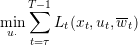
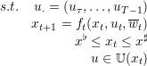
We can now write the optimization criterion:

T∑−1 min 𝔼[ Lt(Pchp,t,FA,t,FN,t,Fth,t+1)] u t=0

(8)

s.t. Bt+1 = Bt + ΔtFB,t B ♭ ≤ Bt ≤ B♯ ♭ ♯ ΔB ≤ Bt+1 −thBt ≤ ΔB Ht+1 = Ht + Δt [(1 − α)Pchp,t + FA,t − Dt♭ + Fth,t+1♯] H ≤ Ht ≤ H

We recall the diﬀerent notations we used previously in Table 1.

State variables
B_t	Battery level	kWh
H_t	Tank level	kWh
Control variables
P_chp,t	CHP power	kW
F_B,t	Energy exchanged with the battery	kW
F_A,t	Production of auxiliary burner	kW
Noises
D_t^el	Electrical demand	kW
D_t^th	Thermal demand	kW
Parameters
π^el	Electricity price	euros
π^gas	Gas price	euros
π^th	Price of uncomfort	euros

Table 1: Notations

2 Simulation and evaluation of given policies

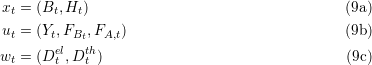
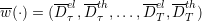
The states, controls and perturbations are now denoted:

We suppose that states belong to a static set x_t ∈ 𝕏, so do control u_t ∈ 𝕌.

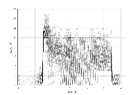
A demand scenarios is a sequence of demands from time t₀ up to T_f − 1.

w(⋅) = (w ,⋅⋅⋅,w ), 0 Tf−1

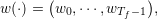(10)

where for all t, w_t = (D_t^el,D_t^th).

w(⋅) is supposed to be the realization of a stochastic process (W_t)_t=0^T_f.

2.1

2.1 Evaluation of a policy

An admissible policy γ : 𝕋 × 𝕏 → 𝕌 assigns a control u = γ(t,x) ∈ 𝕌 to any time t ∈ 𝕋 and to any state x ∈ 𝕏,

Given an admissible policy γ and given a demand scenario w(.) we are able to build trajectories x(⋅) for battery and hot water tank: the dynamic is initiate at time t₀ by:

x0 = xini

and the trajectory is computed step by step with following equation:

We obtain the payoﬀ associated to the demand scenario w(⋅):

γ( ) ∑T J w (⋅) = Lt(xt,ut,wt) t=0

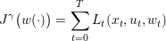(11)

The expected payoﬀ associated with the policy γ is:

( ) 𝔼 Jγ(w (⋅)) ,

(12)

where the expectation 𝔼 is taken with respect to the product probability ℙ. We evaluate (12) by the Monte-Carlo method using N_s scenarios w¹(⋅), ⋅⋅⋅ ,w^N_s(.):

N∑s ( ) -1- J γ ws(⋅) . Ns s=1

(13)

In the next, we will evaluate each algorithm with this method:

We compute trajectories with the help of the function γ given by the algorithm.
We evaluate the average costs with Equation (13).
We consider the distribution of the costs.

The following code generate scenarios that can be used for simulation:

  # Read assessment scenarios:
  De_assess = readcsv("demandelec_assess.csv")
  Dt_assess = readcsv("demandtherm_assess.csv");
  scenarios = zeros(model.stageNumber, 30, 2)
  scenarios[:, :, 1] = De_assess
  scenarios[:, :, 2] = Dt_assess;

The data used for scenarios generation can be obtained here in zip format code.zip or tgz code.tgz.

Question 1

Copy this code and execute it.
Plot 10 scenarios of electrical demand and 10 scenarios of thermal demand.

2.2

2.2 Simulation of a given policy

The function simulate is used to simulate a policy:

  function simulate(scenarios, policy)
      nassess = size(scenarios, 2)
      ntime = size(scenarios, 1)

      x0 = [.6, 20.]
      stocks = zeros(nassess, ntime, 2)
      controls = zeros(nassess, ntime-1, 3)
      costs = zeros(nassess)

      # Set first value of stocks equal to x0:
      for i in 1:nassess
          stocks[i, 1, :] = x0
      end

      for t=1:ntime-1
          for k = 1:nassess
              state_t = stocks[t, k, :]
              aleas = scenarios[t, k, :]

              uc = policy_mpc(t, state_t)

              xf = dynamic(t, state_t, uc, aleas)

              stocks[k, t+1, :] = xf
              controls[k, t, :] = uc
              costs[k] += cost(t, state_t, uc, aleas)
          end
      end

      return costs, stocks, controls
  end

Question 2

What is the inputs of the function simulate? And its outputs?
Relate this function with the theoritical model above.

We consider a ﬁrst policy, given by the echelon-based heuristic:

If the tank’s level is less than a given critical level H^c, then switch on the CHP.
Once the tank is ﬁlled, switch oﬀ the CHP.

Question 3

Implement this heuristic. The function should take as input the time t and the current state x_t and return a control u_t.
Apply this policy along the scenarios generated in Question 1.
Show the costs’ distribution. Plot 10 trajectories for states and controls.

3 Solving by two diﬀerent methods

We are going to compare two policies to solve the problem (8):

a policy produced by the so called Model Predictive Control (MPC),
a policy based upon Dynamic Programming (DP).

We will assess each policy along the scenarios generated in Question 1. However, these policies need to consider some scenarios as input for their algorithms. To be fair, we will use optimization scenarios distinct from the assessment scenarios considered in Question 1.

As we are considering a real world problem, we do not have that much scenarios recorded. That is why we use only 30 scenarios for optimization and 30 scenarios for assessment.

3.1

3.1 Model Predictive Control

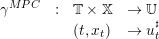
As time goes on, MPC computes at the beginning of each period $[τ,τ + 1[$ the control as a function of the current time and state x_τ. Here are the details:

Derive a deterministic scenario $-- --el -th -el -th w (⋅) = (D τ ,Dτ ,...,DT ,DT )$ of demands (forecast) with the optimization scenarios.
Solve the deterministic optimization problem

T−1 ∑ -- miun⋅ Lt(xt,ut,wt) t=τ

(14)

s.t. u⋅ = (uτ,...,uT−1) xt+1 = ft(xt,ut,wt) x♭ ≤ xt ≤ x♯ u ∈ 𝕌 (xt)

Apply only the ﬁrst control u_τ^{^♯} at time τ, and iterate at time τ + 1

The problem (14) returns a control u_t^{^♯} for all time t and state x_t. This problem gives the MPC policy:

MP C γ : 𝕋× 𝕏 → 𝕌♯ (t,xt) → ut

(15)

γ^MPC is implemented in the function policy_mpc:

  function policy_mpc(t::Int64, x0::Array{Float64})
      tf = NTIME - t

      m = Model()

      # Define constraints other variables:
      @variable(m,  19           <= h[1:(tf+1)]  <= 30)
      @variable(m,  0.5          <= b[1:(tf+1)]  <= 3)
      @variable(m, -DELTA_B_MAX  <= Fb[1:(tf)]   <= DELTA_B_MAX)
      @variable(m,  0.           <= Fa[1:(tf)]   <= 5.5)
      @variable(m,  Fh[1:(tf)]   >=0)
      @variable(m,  0 <= Yt[1:(tf)] <= 1)
      @variable(m,  Z1[1:(tf)] >= 0)


      # Set optimization objective:
      @objective(m, Min, sum{P_BURNER*Fa[i] + P_CHP*Yt[i] +
                             Z1[i] + P_TH*Fh[i], i = 1:tf})

      for i in 1:tf
          @constraint(m, b[i+1] - ALPHA_B * b[i] +
                         DT*BETA_B*Fb[i] == 0)
          @constraint(m, h[i+1] - ALPHA_H * h[i] -
                         DT*BETA_H*(Yt[i]*P_CHP_THERM + Fa[i] -
                         previsions[(i+t -1), 2] + Fh[i]) == 0)

          @constraint(m, Z1[i] >=  (previsions[(i+t -1), 1] -
                                    Fb[i] - Yt[i]*P_CHP_ELEC)*priceElec[t+i-1])
          @constraint(m, Z1[i] >= -(previsions[(i+t -1), 1] -
                                    Fb[i] - Yt[i]*P_CHP_ELEC)*P_INJECTION)
      end

      # Add initial constraints:
      @constraint(m, b[1] == x0[1])
      @constraint(m, h[1] == x0[2])

      status = solve(m)
      return [getvalue(Yt)[1]; getvalue(Fb)[1]; getvalue(Fa)[1]]
  end

Question 4

Explain what the above code is doing.
Apply MPC policy along the scenarios generated in Question 1.
Show the costs’ distribution. Plot 10 trajectories for states and controls.
Does the trajectory of the battery’s state of charge seem reasonable?

3.2

3.2 Stochastic Dynamic Programming

Dynamic programming works in two stages: an oﬄine stage where value functions are computed, and an online stage where these functions are used to compute a policy.

Oﬄine: computation of value functions

Use optimization scenarios to estimate expectation
Use these marginal distributions to compute so-called value functions, given by $[ ( )] Vt(xt) = min 𝔼 Lt(xt,ut,wt)+ Vt+1 ft(xt,ut,wt ) ut∈𝕌$

Online: construction of the policy DP policy computes at the beginning of each period $[τ,τ + 1 [$ the control as a function of the current time τ and state x_τ:

Solve the optimization problem with the help of the previously computed value functions (V _t)_t=0^T_f. $♯ [ ( )] uτ ∈ arugm∈i𝕌n 𝔼 Lt(xτ,uτ,w τ)+ Vτ+1 ft(xτ,uτ,wτ) τ$
Apply control u_τ^{^♯} at time τ, and iterate at time τ + 1.

x_t+1 = f_t(x_t,u_t,w_t) is a functionnal relation, lying in the continuous state space 𝕏. As we use a computer we will discretize state and control spaces to implement dynamic programming. We restrict ourself to a subset 𝕏^d ⊂ 𝕏 for states and 𝕌^d ⊂ 𝕌 for controls.

Implementation The Dynamic Programming solver is already implemented. It is called by the function:

Vs = solve_DP(sdpmodel, paramSDP, 1)

which return the Bellman functions in a multidimensional array Vs.

Question 5 Generate marginal laws with the help of the given optimization scenarios and the function generate_laws.

Question 6

Compute Bellman functions with the function solve_DP.
Apply Dynamic Programming policy along scenarios generated in Question 1.
Show the costs’ distribution. Plot 10 trajectories for states and controls.

Question 7 Plot diﬀerent Bellman functions with the help of the function plot_bellman_functions. Comment the evolution of the shape of these functions along time.

Question 8

Find the discretization used for states and controls. What is the cardinal of the set 𝕏^d (approximation of the space 𝕏)? And those of the set 𝕌^d?
What happens if we reﬁne the discretization of tank and battery by 10?

3.3

3.3 Comparison between diﬀerent policies

We want to compare three diﬀerent features for each algorithm:

the oﬄine computation time,
the online computation time,
the average costs obtained upon the assessment scenarios.

Policy	Oﬄine computation time	Online computation time	Average Costs
Heuristic
MPC
DP

Table 2: Benchmark

Question 9 Fill the Table 2 with the results previously obtained.

A Discretization and interpolation schemes

We have two stocks: a battery and thermal tank. Even if the dynamic programming principle still holds, the numerical implementation is not as straightforward as in the unidimensional case.

A.1

A.1 Discretization

We need to discretize state and control spaces to apply dynamic programming. We restrict ourself to a subset 𝕏^d ⊂ 𝕏 for states and 𝕌^d ⊂ 𝕌 for controls. The policy ﬁnd by dynamic programming is then suboptimal.

To iterate upon diﬀerent states in 𝕏^d, we deﬁne a bijective mapping between 𝕏^d and ℕ. This mapping is written:

d ϕ : 𝕏 → ℕ

(16)

Question 10

Find a mapping that satisfy to the conditions previously stated.
Implement it.

A.2

A.2 Interpolation

With this discretization, we know the value of Bellman function V only upon the grid 𝕏^d, and not upon the whole state 𝕏.

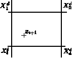
We recall that the next state is given by the state equation: However, even if x_t ∈ 𝕏^d and u_t ∈ 𝕌^d, we can not ensure that x_t+1 ∈ 𝕏^d to compute future cost V _t+1(x_t+1). That is why we need to use an interpolation scheme to interpolate V _t+1(x_t+1) with the values of V _t+1 in 𝕏^d.

Figure 4: x_t+1 could be outside the grid deﬁned by 𝕏^d

Question 11 With the notation introduced in Figure 4, write the linear interpolation of x_t+1 w.r.t X_i^d.

Formations

Départements

Pratique

Recherche

Management of Energy

Management of Renewable Resources and Biodiversity

Management of Exhaustible Resources

Models in Life Science

Miscellaneous