Comparison of stochastic optimization methods

SOWG
(last modiﬁcation date: October 10, 2017)

Version pdf de ce document
Version sans bandeaux

1 Set up
2 Solving the problem
3 Extension

1 Set up
1.1 Problem Presentation
1.2 Setting up the StochDynamicProgramming Library
1.3 Setting up the problem
2 Solving the problem
2.1 Stochastic Dual Dynamic Programming
2.2 Discretized Dynamic Programming
2.3 Extensive Formulation
2.4 Evaluating the solution
3 Extension
3.1 Multi-stock problem
3.2 Display
3.3 Cut Pruning

Abstract

1 Set up

1.1 Problem Presentation

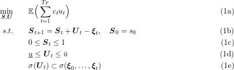
We consider a simple stock management problem over a ﬁnite horizon {1,…,T_F}. The stock follow the dynamic

S = S + U − Xi t+1 t t t

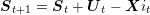
where S_t is the stock at the beginning of time-step t, U_t is the amount of products bought during [t,t + 1[ for a cost c_t, and ξ_t is the amount of product used during [t,t + 1[. We assume that the demand ξ_t is a random exogenous noise with known law over a ﬁnite support. Furthermore we assume a Hazard-Decision setting, where the control U_t is choosen knowing the consumption ξ_t. Finally, we assume bound constraint over the level of stock at each time step and over the control. Thus, the problem reads

1.2 Setting up the StochDynamicProgramming Library

In order to solve the stock management problem using various stochastic optimization approaches we are going to use the StochDynamicProgramming library available in Julia. Julia is an eﬃcient programming language designed for scientiﬁc computing. More information and installation instructions are available at url http://www.julialang.com Installing the library once Julia is installed is easy. Just launch a Julia terminal and type

julia> Pkg.update()
julia> Pkg.add("StochDynamicProgramming")

The ﬁrst line update the list of packages available with their relevant version. The second line add “StochDynamicProgramming” as a required package, and install it as well as all its dependencies packages. All installations are done using git protocol and calling github repositories. In case of trouble you can replace git protocol by https protocol using

git config --global url.https://github.com/.insteadOf git://github.com/

In order to solve the extended formulation of our example, as well as in order to use the SDDP algorithm we will require an external linear solver. If you already have CPLEX or Gurobi installed just type

julia> Pkg.add("CPLEX")

julia> Pkg.add("Gurobi")

Else you can intall a free powerful linear solver with

julia> Pkg.add("Clp")

1.3 Setting up the problem

Once this is done, open (with a text editor) stock-example.jl in the ﬁle examples of your Julia installation

~/.julia/v0.5/StochDynamicProgramming/examples

You can run it with julia stock-example.jl from a terminal launched in the same directory

Let’s comment a few lines of the example.

julia> using StochDynamicProgramming, Clp

This line tell Julia that you are going to use the library StochDynamicProgramming.jl and Clp.jl. The ﬁrst library is a library to model and solve stochastic optimization problems. The second library is a wrapper to the linear solver Clp. It can be replaced by Gurobi or CPLEX if you have them installed on your computer.

  const SOLVER = ClpSolver()    # require "using Clp"
  const MAX_ITER = 10 # number of iterations of SDDP
  const N_STAGES = 6              # number of stages of the SP problem
  const COSTS = [sin(3*t)-1 for t in 1:N_STAGES]
  const CONTROL_MAX = 0.5         # bounds on the control
  const CONTROL_MIN = 0
  const XI_MAX = 0.3              # bounds on the noise
  const XI_MIN = 0
  const N_XI = 10                 # discretization of the noise
  const S0 = 0.5                  # initial stock

These lines deﬁne constant parameters of the problem. You can modify them to test variations of the same problem.

  proba = 1/N_XI*ones(N_XI) # uniform probabilities
  xi_support = collect(linspace(XI_MIN,XI_MAX,N_XI))
  xi_law = NoiseLaw(xi_support, proba)
  xi_laws = NoiseLaw[xi_law for t in 1:N_STAGES-1]

The ﬁrst line deﬁne the probabilities of ξ_t, the second the support of ξ_t. The third line create the actual object representing the random variable. The fourth line state that create the vector (ξ_t)_t. The noises are assumed to be independent.

  function dynamic(t, x, u, xi)
      return [x[1] + u[1] - xi[1]]
  end

This deﬁne the function linking s_t+1 and s_t (see constraint (1b)).

  function cost_t(t, x, u, w)
      return COSTS[t] * u[1]
  end

This function is the current cost to minimize.

  s_bounds = [(0, 1)] # bounds on the state
  u_bounds = [(CONTROL_MIN, CONTROL_MAX)] # bounds on controls
  spmodel = LinearSPModel(N_STAGES,u_bounds,[S0],cost_t,dynamic,xi_laws)
  set_state_bounds(spmodel, s_bounds) # adding the bounds to the model

Finally, these lines deﬁne the spmodel object, which represent our stochastic model including, dynamics, initial state, costs, bounds, and laws of the noises.

2 Solving the problem

Now that the problem is set-up it can be solved through the diﬀerent methods.

2.1 Stochastic Dual Dynamic Programming

  paramSDDP = SDDPparameters(SOLVER,
                              passnumber=10,
                              max_iterations=MAX_ITER)
  V, pbs = solve_SDDP(spmodel, paramSDDP, 2)

The ﬁrst line deﬁne the parameters of the algorithm SDDP. The ﬁrst argument specify the solver required, the second argument the number of forward pass done at each iterations and the third the number of iteration of the SDDP algorithm before stopping. The second line actually solve the problem.

Question 1 Open a Julia terminal. Type

Julia> using StochDynamicProgramming

(auto completion should be working). Then type ’?’ to access the help, and type

help?> solve_SDDP

to obtain a description of the function used here.

Question 2 In the ﬁle stock-example.jl, set run_sdp’, ’run_ef’ and ’test_simulation’ to ’false’ ’.

Modify the example such that:

SDDP run for 20 iterations
SDDP make 5 forward pass

Then run the example either by

julia stock-example

from a bash terminal, or by typing in a julia terminal

julia> include("stock-example.jl")

Remark: in order to navigate from a Julia terminal just type ’;’ and you can use any bash command.

Compare computation time and bounds obtained for multiple values of number of iterations and forward pass.

2.2 Discretized Dynamic Programming

Question 3 Set ’run_sdp’ to ’true’. Run the example to compare the lower bound of sddp and the approximated value of the problem given by sdp.

Test diﬀerent discretization step size (e.g. [0.2,0.1,0.05,0.01]), and compare the computation time and quality of approximation. In theory, how should evolve the computation time with the discretization step ? Do you observe it in practice ?

Question 4 We have solved the problem in Hazard-Decision framework. If the problem was in Decision-Hazard framework, would the value be lower or higher ? Modify the code to check. Don’t forget to revert to hazard-decision before continuing.

2.3 Extensive Formulation

Question 5 Can you determine inequalities between the lower bound of sddp, the value computed by sdp and the value computed by extensive formulation ?

Set ’run_ef’ to ’true’. Numerically check your intuition.

Question 6 Theoretically, how should evolve the computing time of the three methods with N_XI and N_STAGES ? Numerically test your intuition by increasing / decreasing the parameters N_XI and N_STAGES.

2.4 Evaluating the solution

Once we have obtained the solution to our problem we would like to simulate the strategy obtained and evaluate the costs.

Question 7 Simulate the strategies obtained by sddp over 1000 scenarios. Print the mean cost obtained by each strategy, and the relative diﬀerence. Compare to the lower bound of sddp, the value given by sdp and the value given by extensive formulation. Repeat 10 times and comment.

Question 8 Fix the random seed, compare the quality of the solution obtained with various parameters of sddp and sdp on the same scenarios.

3 Extension

We present here a few extensions to manipulate the package.

3.1 Multi-stock problem

The example ’multistock-example.jl’ is extremely close to ’stock-example.jl’ but incorporate multiple stocks linked through a constraint on the controls.

Question 9 Theoretically what is the computing time dependence in the parameter ’step’ ? Test it by setting step to 0.05 and 0.2. Comment on the quality of the solution.

Question 10 Theoretically what is the computing time dependence in the parameter N_STAGES ? Test it.

Question 11 Theoretically what is the computing time dependence in the parameter N_STOCKS ? Test it.

Question 12 Theoretically what is the computing time dependence in the parameter N_XI ? Test it.

3.2 Display

In a Julia terminal in the example directory.

julia> include("display.jl")
julia> include("stock-example.jl")

Question 13 Plot the cost distribution of SDDP and SDP.

Question 14 Plot some optimal trajectories of stocks.

3.3 Cut Pruning

A cut pruning method is available in the package and can be used as follows.

  paramSDDP_pruned = SDDPparameters(SOLVER,
                                 passnumber=10,
                                 max_iterations=MAX_ITER,
                                 pruning_algo="exact",
                                 prune_cuts = 1)

The parameter pruning_algo can be set to the string value "exact" or to to the string value "level1". The prune_cuts parameter is used to deﬁne at which periodicity the pruning method must be applied.

Question 15 test the pruning on the stock example and make comments on the computing time eﬃciency.

Formations

Départements

Pratique

Recherche

Management of Energy

Management of Renewable Resources and Biodiversity

Management of Exhaustible Resources

Models in Life Science

Miscellaneous