


| L'École des Ponts ParisTech est membre fondateur de |
L'École des Ponts ParisTech est certifiée |


|
|


Consider a renewable ressource whose stock, measured through its biomass B, is considered globally, as one single unit, without any consideration for the structure population. Its growth is materialized through the linear Schaefer model
 | (1) |
where h(t) is the harvesting at time t and R(t) = 1 + r(t) is the productivity of the resource.
Adapted from [1, p. 258], we shall illustrate the results with the Antartic baleen whale example as in Table 1.
| Antartic baleen whale | |
| intrinsic growth | r = 5% |
| carrying capacity | K = 400 000 BWH |
| catchability | q = 0.0 016 WCY |
| price | p = 7 000 $ per BWU |
| cost | c = 600 000 $ per WCY |
In this case, the productivity is stationary and deterministic:
 | (2) |
Question 1 You have to manage the whale population whose dynamics parameters are given in Table 1. Design your own catch strategy Catch(t,B) (following the model of the random catch effort strategy in the scilab code below). Give the scilab code corresponding to your own catch strategy. Draw simulations of biomass and catch trajectories.
We now assume that some planner aims at maximizing the sum of discounted utilities of the catches plus a final stock utility. The maximization problem is
 | (3) |
where ρ =  ∈ [0, 1] is a discount factor and Util(⋅) is a utility function, concave and
strictly increasing on ℝ+. Notice that the final term Util
∈ [0, 1] is a discount factor and Util(⋅) is a utility function, concave and
strictly increasing on ℝ+. Notice that the final term Util B(T)
B(T) corresponds to an
existence or inheritance value of the stock. We shall use a discount factor ρ with typical
values ranging between 0.9 and 1. We restrict the study to the isoelastic utility case
where
corresponds to an
existence or inheritance value of the stock. We shall use a discount factor ρ with typical
values ranging between 0.9 and 1. We restrict the study to the isoelastic utility case
where
 | (4) |
The dynamic programming equation is:
 | (5) |
By backward induction, it can be proved that
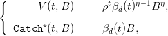 | (6) |
where βd(t) is given by the backward equation
 | (7) |
It can be deduced that, along the optimal path given by
 | (8) |
we have
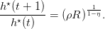 | (9) |
Question 2 Simulate optimal catches and biomass trajectories (B⋆(t),h⋆(t)). Change the value of the discount factor ρ to modify the location of ρR with respect to 1. Do at least three cases with ρR > 1, ρR = 1 and ρR < 1. What do you observe?
Question 3 What is the influence of η on the optimal paths (B⋆(t),h⋆(t))? In particular, what happens when η ≈ 1? Comment knowing that 1 − η may be interpreted as the constant relative risk aversion of the decision-maker.
Question 4 Write a program which evaluates the criterion
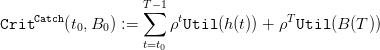 | (10) |
for any catch decision rule Catch : (t,B) Catch(t,B) (admissible in the sense that
0 ≤ Catch(t,B) ≤ B), and where
Catch(t,B) (admissible in the sense that
0 ≤ Catch(t,B) ≤ B), and where
 | (11) |
Compare the criterion values given by
Question 5 Write a program which computes for any harvesting strategy Catch(t,B)
Plot and compare the profit trajectories t profit(t) given by
We now assume that the planner aims at sustainability and intergenerational equity, and attempts at maximizing the utility of the “poorest” generation. The maximization problem is then
 | (14) |
The dynamic programming equation is:
 | (15) |
By backward induction, it can be proved that
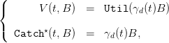 | (16) |
where γd(t) is given by the backward equation
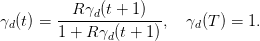 | (17) |
Consequently, along the maximin optimal path given by
 | (18) |
we have
 | (19) |
Question 6 Adapt the previous scilab code to obtain the maximin path (B⋆(t),h⋆(t)).
Question 7 Compare the trajectories of the maximin criterion, of the stock biomasses and of the catches between
We assume that the policy is to constrain the biomass level within an ecological window, namely between conservation and maximal safety values:
 | (20) |
A minimal catch is also required:
 | (21) |
The dynamic programming equation for the viability kernels is:
![(
{ V iab(T) = [B♭,B ♯],
( V iab(t) = {B ∈ [B ♭,B♯] | ∃h ∈ [h♭,B], R (B − h) ∈ V iab(t + 1)}.](Resource_management26x.png) | (22) |
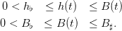
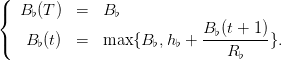
Question 8 Define by backward induction
Show that, whenever B♭(t) ≤ B♯, the viability kernels are intervals:
![V iab(t) = [B ♭(t),B ♯].](Resource_management28x.png)
Show that the viable decision rules Catch(t,B) are those which belong to
![[h♭(t,B),h ♯(t,B )] := [B − B-♯,B − B-♭(t +-1)].
R R](Resource_management29x.png)
Question 9 Fix a guaranteed yield h♭ as a fraction of carrying capacity K. Simulate trajectories with different viable decision rules.
The maximization problem is
 | (23) |
under the contraints
The dynamic programming equation is:
 | (24) |
The maximization problem is
 | (25) |
under the contraints
The dynamic programming equation is:
 | (26) |
The R(t) vary in an interval [R♭,R♯].
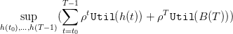
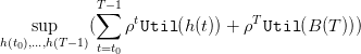
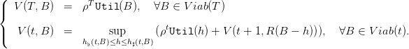
The maximization problem is
![T−1
sup inf (∑ ρtUtil (h(t)) + ρT Util (B (T ))).
h(t0),...,h(T−1)R(⋅)∈[R ♭,R♯]T+1
t=t0](Resource_management36x.png) | (27) |
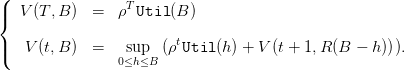
The dynamic programming equation is:
![(
|{ V (T,B ) = ρTUtil (B ),
|( V (t,B ) = sup inf (ρtUtil (h) + V (t + 1,R (B − h))).
0≤h ≤BR ∈[R♭,R♯]](Resource_management37x.png) | (28) |
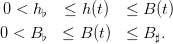
We restrict the study to the isoelastic case (4).
The maximization problem is
![sup inf min( min Util (h(t)),Util(B (T))).
h(t0),...,h(T−1)R(⋅)∈[R♭,R♯]T+1 t=t0,...,T−1](Resource_management38x.png) | (29) |
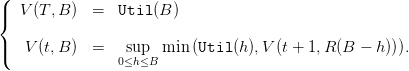
The dynamic programming equation is:
![(| V (T,B ) = Util (B )
{
|( V(t,B ) = 0s≤uhp≤B R∈[inRf♭,R ♯]min (Util (h),V (t + 1,R (B − h ))).](Resource_management39x.png) | (30) |
We assume that the policy is to constrain the biomass level within an ecological window, namely between conservation and maximal safety values, whatever the scenario:
 | (31) |
A minimal catch is also required:
 | (32) |
The dynamic programming equation for the robust viability kernels is:
![(
{ Viab1(T ) = [B♭,B ♯],
( V iab (t) = {B ∈ [B ,B ] | ∃h ∈ [h ,B ],∀R ∈ [R ,R ],R (B − h ) ∈ V iab (t + 1)}.
1 ♭ ♯ ♭ ♭ ♯ 1](Resource_management42x.png) | (33) |
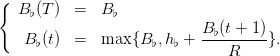
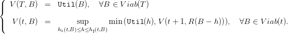
Question 16 Define by backward induction
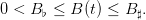
Show that, whenever
the viability kernels are intervals:
![V iab(t) = [B ♭(t),B ♯].](Resource_management45x.png)
Show that the viable decision rules Catch(t,B) are those which belong to
![[h♭(t,B),h ♯(t,B )] := [B − B-♯,B − B-♭(t +-1)].
R ♯ R ♭](Resource_management46x.png)
| L'École des Ponts ParisTech est membre fondateur de |
L'École des Ponts ParisTech est certifiée |
|
|
|


