Contents

1 Prerequisite Scilab code

You will have to fill the following skeleton of scilab code during the practical course.

• dam_management2.sce

2 Problem statement

We consider a dam manager intenting to maximize the intertemporal payoff obtained by selling power produced by water releases.

2.1 Dam dynamics

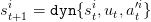
Consider the dam dynamics s_t+1 = dyn, where

(1)

where

• time t ∈ [[t₀,T]] is discrete (such as days, weeks or months),
• s_t is the stock level (in water volume) at the beginning of period [t,t + 1[, belonging to 𝕊 = [[s,s]], where s and s are the minimum and maximum volume of water in the dam,
• the variable u_t is the control decided at the beginning of period [t,t + 1[ belonging to (it can be seen as the period during which the turbine is open, and the effective water release is min{s_t + a_t,u_t}, necessarily less than the water s_t + a_t in the dam at the moment of turbinating),
• a_t is the water inflow (rain, hydrology, etc.) during the period [t,t + 1[.

2.2 Intertemporal payoff criterion

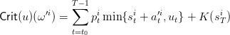
We consider a problem of payoff maximization where turbining one unit of water has unitary price p_t. On the period from t₀ to T, the payoffs sum up to

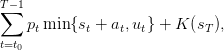(2)

where K is the final valorization of the water in the dam.

2.3 Uncertainties and scenarios

Both the inflows a_t and the prices p_t are uncertain variables. We denote by w_t := (a_t,p_t) the couple of uncertainties at time t. A scenario

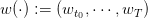(3)

is a sequence of uncertainties, inflows and prices, from initial time t₀ up to the horizon T.

2.4 Generation of trajectories and payoff by a policy

A policy ϕ : [[t₀,T − 1]] × 𝕊 → 𝕌 assigns a control to any state s of dam stock volume and to any time t ∈ [[t₀,T − 1]].

Given a policy ϕ and a scenario w(⋅) as in (3), we obtain a volume trajectory 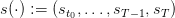and a control trajectory 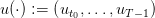produced by the “closed-loop” dynamics

(4)

Pluging the trajectories and given by (4) in the criterion (2), we obtain the evaluation

(5)

2.5 Numerical data

We consider a weekly management over a year, that is t₀ = 0 and T = 52, with

(6)

Prices and inflows data can be downloaded using the following html links:

• dam_prices_52.txt
• dam_intakes_52.txt

3 Evaluation of a strategy

We begin by generating a scenario of inflows and prices as follows.

Then, we are going to implement the code corresponding to §2.4 under the form of a macro simulation_det whose input arguments are a scenario and a policy (itself given under the form of a macro with two inputs and one output).

This done, we are going to test the above macro simulation_det with simple strategies.

4 Optimization in a deterministic setting

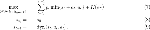
In a deterministic setting, we consider that the sequences of prices p(⋅) and inflows w(⋅) are known, and we optimize accordingly. The optimization problem we consider is

The theoretical Dynamic Programming equation is

(10)

4.1 Zero final value of water

Here, we fix the final value K of water in problem (7) to 0. This means that the water remaining in the dam at time T presents no economic interest for the manager.

4.2 Determining the final value of water

We are optimizing the dam on one year. However at the end of this year the dam manager will still have to manage the dam, thus the more water in the dam at the end, the better for the next year. The question is how to determine this value.

The main idea is the following : we want to optimize the management of our dam on a very long time, however we would like to actually solve the problem only on the first year, representing the remainings years by the final value function K in (7). Thus K(s) should represent how much we are going to earn during the remaining time, starting at state s.

Thus, choosing the final value K = K_N means that we take in consideration the gains on N years. We would like to have N going to infinity, however K_N+1 − K_N is more or less the gain during one year, thus K_N will not converge. In the following question we will find a way of determining a final value converging with N that represents the problem on a long time.

4.3 Introducing a constraint on the water level during summer months

For environemental and touristic reasons the level of water in the dam is constrained. We expect that, during the summer months (week 25 to 40), the level of water in the dam must be above a minimal level s′.

4.4 Closed-loop vs open-loop control

A closed-loop strategy is a policy given by ϕ : [[t₀,T − 1]] × 𝕊 → 𝕌, which assigns a water turbined to any state s of dam stock volume and to any decision period t ∈ [[t₀,T − 1]], whereas an open-loop strategy is a predetermined planning of control, that is a function ϕ : [[t₀,T − 1]] → 𝕌.

Let us note that, formally, an open-loop strategy is a closed-loop strategy.

However, one can make an error in his prediction on inflows or prices and open-loop control may suffer from this. In order to represent this, we will proceed in the following way.

1. We simulate a scenario of prices and inflows.
2. We determine the optimal closed-loop strategy via Dynamic Programming.
3. We determine the associated optimal open-loop strategy.
4. We test both strategies on the original scenario.
5. We modify slightly the original scenario (keep in mind that all inflows must be integers)
6. We test both strategies on the modified scenario.

The “slight” modification of the original scenario must be simple and well understood. Thus we should change either the price or the inflow, at a few times only. However the size of the modification can be substantial.

5 Optimization in a stochastic setting

In section 3 we have made optimization and simulation on a single scenario. However water inflows and prices are uncertain, and we will now take that into account.

5.1 Probabilistic model on water inputs and expected criterion

We suppose that sequences of uncertainties , are discrete random variables with known probability distribution. Moreover we will assume that a(⋅) and p(⋅) are independent, and that each of them is a sequence of independent random variables.

Notice that the random variables are independent, but that they are not necessarily identically distributed. This allows us to account for seasonal effects (more rain in autumn and winter).

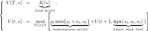
To each strategy ϕ, we associate the expected payoff

(11)

This expected payoff will be estimated by a Monte-Carlo approach. In order to do that we will use the macros Price and Inflows that generate a table of random trajectories of the noise, each line being one scenario. The expected payoff of one strategy will be estimated as the empirical mean of the payoff on these scenarios. In order to compare two strategies we have to use the same scenarios for the Monte-Carlo estimation. Thus, we fix a set of simulation scenarios (ω_i)_i∈[[1,n]], where ω_i = {p₁ⁱ,a ₁ⁱ,,p _T ⁱ,a _T ⁱ}. and we will always evaluate the criterion 𝔼Crit^ϕ as ∑ _i=1^NCrit^ϕ(ω _i).

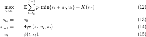
Consequently the problem is now written as

5.2 Simulation of strategies in a stochastic setting

Here, we will use the macros simulation and simulation_Bellman that simulate a strategy on each scenario giving a vector of gains, as well as a matrix of stock and control trajectories.

5.3 Open-loop control of the dam in a probabilistic setting

We have seen that, in the deterministic case (without any errors of prevision), an open-loop strategy is equivalent to a closed-loop strategy. Thus, in a probabilistic setting, one can be tempted to determine an optimal open-loop strategy.

In a first part, we will work on a mean scenario to derive an open-loop strategy.

In a second part we compute the best open-loop strategy using the function optim built-in in Scilab. We choose a set of optimization scenarios (ω′_i)_{i∈[[1,Nmc]]}, where ω′_i = {p′₁ⁱ,a′ ₁ⁱ,,p′ _T ⁱ,a′ _T ⁱ}. (let us note that this set of scenarios is fixed and that it is different from the set of simulation scenarios). Then we construct a cost function J(u) as

where u is a vector of T − 1 variables reprensenting the planning of control. Thus we have

with

5.4 Stochastic Dynamic Programming Equation

5.4.1 Decision-Hazard framework

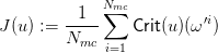
We will now focus on finding an optimal closed loop solution for problem (12) The dynamic programming equation associated to the problem of maximizing the expected profits is

(16)

5.4.2 Hazard-Decision framework

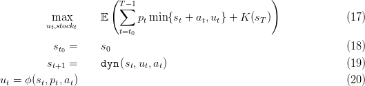
One may note that, in practice, the dam manager often assume that the weekly inflows and prices are perfectly known. Indeed at the beginning of the week meteorologists and economists can give some predictions. Moreover this problem is only an approximation of the real one, as a dam is managed per hour and not per week, thus the manager has more information than what we assume in a Decision-Hazard setting. Consequently we will now change slightly problem (12) by assuming that, at each time step t we know the price p_t and inflow a_t.

Problem (12) is turned into

5.5 (Anticipative) upper bound for the payoff

The choice of the probabilistic model of noises (prices and inflows) is quite important. Until now, we have represented the noises as independent variables, and this is not the more precise probabilistic model we could have used. Consequently we might want to estimate the potential gain in using a more precise (but numerically less tractable) probabilistic model. Thus we would like to have an upper bound on our problem. Such an upper bound can be found by doing an anticipative study : for each scenario we compute the best possible gains on this scenario.

Let us stress out that this will not give a strategy that can be used. It only gives an upper bound on the possible gain for a set of simulation scenario, a-posteriori.

6 Correction

• dam_management2_correction.sce