Viable Harvesting of a Renewable Resource

Luc Doyen, Michel De Lara
(last modiﬁcation date: October 10, 2017)

Version pdf de ce document
Version sans bandeaux

1 The modelling
2 The viability result
3 The Beverton-Holt case
4 Another population dynamics

1 The modelling
2 The viability result
3 The Beverton-Holt case
3.1 Dynamics and equilibrium
3.2 The unsustainable case: 𝕍iab = ∅
3.3 The sustainable case: 𝕍iab ⁄= ∅
4 Another population dynamics

1 The modelling

Let us consider some regulating agency aiming at the sustainable use and harvesting of a renewable resource. The biomass of this resource at time t is denoted by B(t) while the harvesting level is h(t). We assume that the natural dynamics is described by some growth function Biol. Under exploitation, the following controlled dynamics is obtained for t ∈ ℕ

B (t + 1) = Biol(B (t) − h (t))

(1)

with the admissibility constraint

0 ≤ h(t) ≤ B(t).

(2)

The policy goal is to guarantee at each time a minimal harvesting

hlim ≤ h(t),

(3)

together with a non extinction level for the resource

Blim ≤ B (t).

(4)

The combination of constraints (2) and (3) yields the state constraint

hlim ≤ B(t).

(5)

For the sake of simplicity, we assume that h_lim > B_lim.

2 The viability result

We use the viability approach to handle the problem. We aim at “showing” and recovering numerically the characterization of the viability kernel described in Result 1. We introduce the following notations.

The sustainable yield function Sust is deﬁned by
$h = Sust (B ) ⇐ ⇒ B = Biol (B − h) and 0 ≤ h ≤ B.$ (6)
The maximum sustainable biomass B_MSE and maximum sustainable yield h_MSE are deﬁned by
$hMSE = Sust (BMSE ) = max Sust (B ). B ≥0$ (7)
When h_lim ≤ h_MSE, the viability barrier B_V is the solution of
$BV = min B. B,hlim=Sust(B)$ (8)

Result 1 Assume that Biol is an increasing continuous function on ℝ₊. The viability kernel is characterized by

{ [BV ,+ ∞ [ if hlim ≤ hMSE 𝕍iab = ∅ otherwise.

(9)

Viable controls are those h (depending on B) such that

Biol (B − h) ∈ [BV ,+ ∞ [ and 0 ≤ h ≤ B.

(10)

3 The Beverton-Holt case

3.1 Dynamics and equilibrium

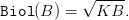
We consider the natural evolution governed by

-RB---- Biol (B ) = 1 + bB .

(11)

For numerical computations and simulations, we consider the case of the Paciﬁc yellowﬁn tuna, with intrinsic growth R = 2.25 metric tons per year and carrying capacity K = 250 000 metric tons. Since the carrying capacity solves Biol(K) = K, we obtain

R = 2.25 metric tons per year and b = R-−-1-= 5 10−6 (metric tons per year)− 1. K

(12)

Question 1

Deﬁne a Scilab function for the dynamics Biol in (11), and a Scilab function for the equilibrium harvesting h = Sust(B) deﬁned in (6).
Plot the sustainable yield function BSust(B).
Compute the maximum sustainable population equilibrium B_MSE and the maximum sustainable yield h_MSE.

  // Population dynamics parameters
  R_tuna=2.25;
  R=R_tuna;
  K_tuna=250000;// carrying capacity
  K=K_tuna;

  // BEVERTON-HOLT DYNAMICS
  b=(R-1)/K;

  function y=dynamics(B) y=R*B ./(1+b*B);endfunction

  function h=SY(B) h=B-(B ./(R-b*B));endfunction

  B_MSE=(R-sqrt(R))/b;
  disp('The maximum sustainable population equilibrium is '+string(B_MSE)+ ...
       ' metric tons (MT)');

  h_MSE=SY(B_MSE);
  disp('The maximum sustainable yield is '+string(h_MSE)+' metric tons (MT)');

  xset("window",10);xbasc();
  // xbasc() is no longer valid with scilab, but works with scicos
  abcisse_B=linspace(0,K,20);
  plot2d(abcisse_B,SY(abcisse_B))
  xtitle('Sustainable yield associated to Beverton-Holt dynamics','biomass (MT)', ...
         'yield (MT)');

3.2 The unsustainable case: 𝕍iab = ∅

Question 2

Choose a guaranteed harvesting h_lim strictly larger than Sust(B_MSE).
For several initial conditions B₀, compute diﬀerent trajectories for the smallest admissible harvesting, namely h(t) = h_lim.
What happens with respect to viability constraint (5)?
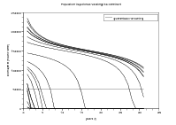
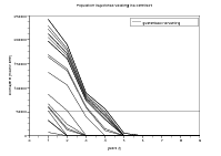
Show that the situation is more catastrophic with sequences of harvesting h(t) larger than the guaranteed one h_lim. Try for instance admissible policies:
- h(t,B) = B;
- h(t,B) = αh_lim + (1 − α)B with α ∈ [0, 1] (see Figure 1(a));
- h(t,B) = α(t)h_lim+(1−α(t))B, where (α(t))_t∈ℕ is an i.i.d. sequence of uniform random variables in [0, 1] (see Figure 1(b)).

  // number of random initial conditions
  nbsimul=20;
  // The unsustainable case:
  h_lim=(1+rand()/5)*h_MSE

  Horizon=30;
  years=1:Horizon;
  yearss=[years,years($)+1];
  traj_B=[];

  xset("window",11);xbasc();

  for i=1:nbsimul do
    traj_B(1)=K*rand(1);
    for t=years do
      traj_B(t+1)=max(0,dynamics(traj_B(t)-h_lim));
      // max is no longer valid with scilab (use maxi), but works with scicos
    end,
    plot2d(yearss,traj_B);
  end,
  plot2d(yearss,h_lim*ones(yearss))
  xtitle('Population trajectories violating the constraint','years (t)', ...
         'biomass B (metric tons)')
  legends('guaranteed harvesting',1,'ur')

  /////////////////////////////////////////////////

  function h=policy(t,B,alpha)
    h=max(h_lim,alpha*h_lim+(1-alpha)*B);
  endfunction

  Horizon=8;
  years=1:Horizon;
  yearss=[years,years($)+1];
  traj_B=[];
  traj_h=[];
  alpha=rand(years);

  xset("window",12);xbasc();

  for i=1:nbsimul do
    traj_B(1)=K*rand(1);
    for t=years do
      traj_h(t)=policy(t,traj_B(t),alpha(t));
      traj_B(t+1)=max(0,dynamics(traj_B(t)-traj_h(t)));
    end,
    plot2d(yearss,traj_B);
  end,
  plot2d(yearss,h_lim*ones(yearss))
  xtitle('Population trajectories violating the constraint','years (t)', ...
         'biomass B (metric tons)')
  legends('guaranteed harvesting',1,'ur')

(a) Population viability constraint violated (stationary harvesting)

(b) Population viability constraint violated (random harvesting)

Figure 1: Biomass trajectories violating the viability state constraint (5) (horizontal line at h_lim)

3.3 The sustainable case: 𝕍iab≠∅

Question 3

Now choose a guaranteed harvesting h_lim strictly smaller than h_MSE = Sust(B_MSE).
Compute the viability barrier B_V.
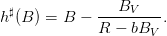
Prove that the viable policies are those h(t,B) which lie within the set [h_lim,h^♯(B)] where
$h♯(B ) = B − ---BV----. R − bBV$ (13)
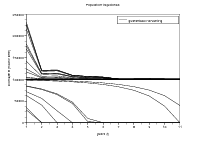
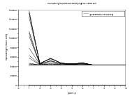
For diﬀerent initial conditions B₀, compute diﬀerent trajectories for a harvesting policy of the form
$♯ h (t,B ) = α(t)hlim + (1 − α (t))h (B ).$ (14)
What happens with respect to viability constraint (5)? See Figure 2.

  // The sustainable case
  h_lim=(1-rand()/5)*h_MSE
  /////////////////////////////////////////////////
  // numerical estimation of the viability barrier
  function residual=viabbarrier(B)
    residual=SY(B)-h_lim
  endfunction

  B_V=fsolve(0,viabbarrier)
  /////////////////////////////////////////////////
  function h=h_max(B)
    h=B-(B_V/(R-b*B_V))
  endfunction

  function h=viab(t,B,alpha)
    h=max(h_lim,alpha*h_lim+(1-alpha)*h_max(B));
  endfunction

  Horizon=10;
  years=1:Horizon;
  yearss=[years,years($)+1];

  xset("window",21);xbasc();
  xtitle('Population trajectories ','years (t)','biomass B (metric tons)')
  traj_B=[];

  xset("window",22);xbasc();
  xtitle("Harvesting trajectories satisfying the constraint",'years (t)', ...
         'harvesting h (metric tons)')
  traj_h=[];

  alpha=rand(years);

  for i=1:nbsimul do
    traj_B(1)=K*rand(1);
    for t=years do
      traj_h(t)=viab(t,traj_B(t),alpha(t));
      traj_B(t+1)=max(0,dynamics(traj_B(t)-traj_h(t)));
    end,
    xset("window",21);plot2d(yearss,traj_B);
    plot2d(yearss,B_V*ones(yearss));
    legends('viability barrier',1,'ur')
    //
    xset("window",22);plot2d(years,traj_h);
    plot2d(years,h_lim*ones(years));
    legends('guaranteed harvesting',1,'ur')
    plot2d(years,0*ones(years));
    // for the scale
  end

(a) Population viability constraint satisﬁed or violated

(b) Minimal guaranteed harvesting viability constraint satisﬁed

Figure 2: Population trajectories violating or satisfying the viability state constraint (5), depending whether the original biomass is lower or greater than the viability barrier (horizontal line at B_V). Harvest trajectories satisfying the minimal harvesting viability constraint (3) (horizontal line at h_lim).

4 Another population dynamics

The natural evolution is now governed by

√ ---- Biol(B ) = KB.

(15)

sqrt(max(0,K*B))

Question 4 Do the same as in the previous Beverton-Holt case.

Formations

Départements

Pratique

Recherche

Management of Energy

Management of Renewable Resources and Biodiversity

Management of Exhaustible Resources

Models in Life Science

Miscellaneous